图像分割

图像分割模型将图像中对应不同感兴趣区域的区域分离出来。这些模型通过为每个像素分配一个标签来工作。分割有几种类型：语义分割、实例分割和全景分割。

在本指南中，我们将：

了解不同类型的分割。
提供一个用于语义分割的端到端微调示例。

在开始之前，请确保已安装所有必要的库：

# uncomment to install the necessary libraries
!pip install -q datasets transformers evaluate accelerate trackio

我们建议您登录您的 Hugging Face 账户，以便上传并与社区共享您的模型。当系统提示时，请输入您的令牌以完成登录：

>>> from huggingface_hub import notebook_login

>>> notebook_login()

分割的类型

语义分割为图像中的每个像素分配一个标签或类别。让我们来看一个语义分割模型的输出。它会将图像中同一物体的所有实例分配为相同的类别，例如，所有的猫都会被标记为“cat”，而不是“cat-1”、“cat-2”。我们可以使用 transformers 的图像分割流水线来快速推理语义分割模型。让我们来看一个示例图像。

from transformers import pipeline
from PIL import Image
import requests

url = "https://huggingface.co/datasets/huggingface/documentation-images/resolve/main/transformers/tasks/segmentation_input.jpg"
image = Image.open(requests.get(url, stream=True).raw)
image

我们将使用 nvidia/segformer-b1-finetuned-cityscapes-1024-1024。

semantic_segmentation = pipeline("image-segmentation", "nvidia/segformer-b1-finetuned-cityscapes-1024-1024")
results = semantic_segmentation(image)
results

分割流水线的输出包含每个预测类别对应的掩码。

[{'score': None,
  'label': 'road',
  'mask': <PIL.Image.Image image mode=L size=612x415>},
 {'score': None,
  'label': 'sidewalk',
  'mask': <PIL.Image.Image image mode=L size=612x415>},
 {'score': None,
  'label': 'building',
  'mask': <PIL.Image.Image image mode=L size=612x415>},
 {'score': None,
  'label': 'wall',
  'mask': <PIL.Image.Image image mode=L size=612x415>},
 {'score': None,
  'label': 'pole',
  'mask': <PIL.Image.Image image mode=L size=612x415>},
 {'score': None,
  'label': 'traffic sign',
  'mask': <PIL.Image.Image image mode=L size=612x415>},
 {'score': None,
  'label': 'vegetation',
  'mask': <PIL.Image.Image image mode=L size=612x415>},
 {'score': None,
  'label': 'terrain',
  'mask': <PIL.Image.Image image mode=L size=612x415>},
 {'score': None,
  'label': 'sky',
  'mask': <PIL.Image.Image image mode=L size=612x415>},
 {'score': None,
  'label': 'car',
  'mask': <PIL.Image.Image image mode=L size=612x415>}]

观察汽车类别的掩码，我们可以看到每辆汽车都被分配了相同的掩码。

results[-1]["mask"]

在实例分割中，目标不是对每个像素进行分类，而是为给定图像中每个物体实例预测一个掩码。它与目标检测非常相似：目标检测中每个实例都有一个边界框，而这里则使用分割掩码。我们将使用 facebook/mask2former-swin-large-cityscapes-instance 来完成此任务。

instance_segmentation = pipeline("image-segmentation", "facebook/mask2former-swin-large-cityscapes-instance")
results = instance_segmentation(image)
results

如下所示，存在多个被分类的汽车，并且除了属于汽车和行人实例的像素外，其他像素均没有分类。

[{'score': 0.999944,
  'label': 'car',
  'mask': <PIL.Image.Image image mode=L size=612x415>},
 {'score': 0.999945,
  'label': 'car',
  'mask': <PIL.Image.Image image mode=L size=612x415>},
 {'score': 0.999652,
  'label': 'car',
  'mask': <PIL.Image.Image image mode=L size=612x415>},
 {'score': 0.903529,
  'label': 'person',
  'mask': <PIL.Image.Image image mode=L size=612x415>}]

查看下方其中一个汽车掩码。

results[2]["mask"]

全景分割结合了语义分割和实例分割，其中每个像素都被分类到一个类别以及该类别的一个实例，并且每个类别的每个实例都有多个掩码。我们可以使用 facebook/mask2former-swin-large-cityscapes-panoptic 来实现这一点。

panoptic_segmentation = pipeline("image-segmentation", "facebook/mask2former-swin-large-cityscapes-panoptic")
results = panoptic_segmentation(image)
results

如下所示，我们有更多的类别。稍后我们将展示如何对每个像素进行分类，使其归属于其中一个类别。

[{'score': 0.999981,
  'label': 'car',
  'mask': <PIL.Image.Image image mode=L size=612x415>},
 {'score': 0.999958,
  'label': 'car',
  'mask': <PIL.Image.Image image mode=L size=612x415>},
 {'score': 0.99997,
  'label': 'vegetation',
  'mask': <PIL.Image.Image image mode=L size=612x415>},
 {'score': 0.999575,
  'label': 'pole',
  'mask': <PIL.Image.Image image mode=L size=612x415>},
 {'score': 0.999958,
  'label': 'building',
  'mask': <PIL.Image.Image image mode=L size=612x415>},
 {'score': 0.999634,
  'label': 'road',
  'mask': <PIL.Image.Image image mode=L size=612x415>},
 {'score': 0.996092,
  'label': 'sidewalk',
  'mask': <PIL.Image.Image image mode=L size=612x415>},
 {'score': 0.999221,
  'label': 'car',
  'mask': <PIL.Image.Image image mode=L size=612x415>},
 {'score': 0.99987,
  'label': 'sky',
  'mask': <PIL.Image.Image image mode=L size=612x415>}]

让我们对所有类型的分割进行并排比较。

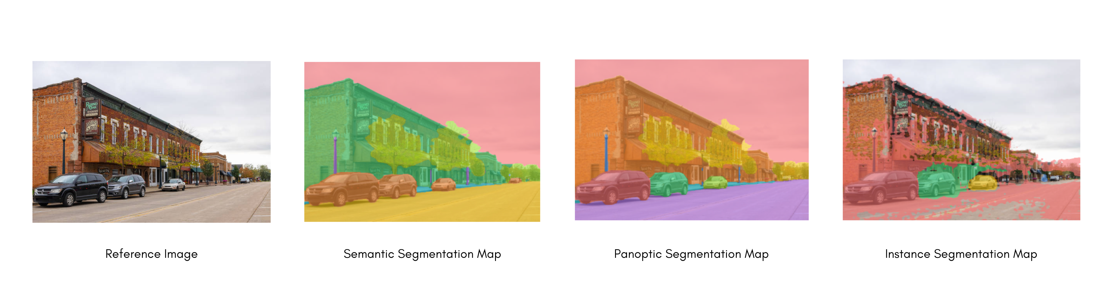
在了解了各种类型的分割之后，让我们深入探讨如何针对语义分割微调模型。

语义分割在现实世界中的常见应用包括：训练自动驾驶汽车以识别行人和重要的交通信息、在医学影像中识别细胞和异常，以及通过卫星图像监测环境变化。

用于分割任务的模型微调

我们将执行以下操作：

在 SceneParse150 数据集上微调 SegFormer。
使用您微调后的模型进行推理。

要查看与此任务兼容的所有架构和检查点，我们建议查阅任务页面

加载 SceneParse150 数据集

首先，从 🤗 Datasets 库中加载 SceneParse150 数据集的一个较小子集。这将让你有机会进行实验，确保一切正常运行，然后再花更多时间在完整数据集上进行训练。

>>> from datasets import load_dataset

>>> ds = load_dataset("merve/scene_parse_150", split="train[:50]")

使用 train_test_split 方法将数据集的 train 子集拆分为训练集和测试集：

>>> ds = ds.train_test_split(test_size=0.2)
>>> train_ds = ds["train"]
>>> test_ds = ds["test"]

然后来看一个示例：

>>> train_ds[0]
{'image': <PIL.JpegImagePlugin.JpegImageFile image mode=RGB size=512x683 at 0x7F9B0C201F90>,
 'annotation': <PIL.PngImagePlugin.PngImageFile image mode=L size=512x683 at 0x7F9B0C201DD0>,
 'scene_category': 368}

# view the image
>>> train_ds[0]["image"]

image：场景的 PIL 图像。
annotation：分割掩码的 PIL 图像，同时也是模型的目标。
scene_category：描述图像场景的类别 ID，例如“kitchen”或“office”。在本指南中，你只需要 image 和 annotation，它们都是 PIL 图像。

您还需要创建一个将标签 ID 映射到标签类别的字典，这在后续设置模型时会很有用。从 Hub 下载映射，并创建 id2label 和 label2id 字典：

>>> import json
>>> from pathlib import Path
>>> from huggingface_hub import hf_hub_download

>>> repo_id = "huggingface/label-files"
>>> filename = "ade20k-id2label.json"
>>> id2label = json.loads(Path(hf_hub_download(repo_id, filename, repo_type="dataset")).read_text())
>>> id2label = {int(k): v for k, v in id2label.items()}
>>> label2id = {v: k for k, v in id2label.items()}
>>> num_labels = len(id2label)

预处理

下一步是加载 SegFormer 图像处理器，以将图像和标注准备好供模型使用。一些数据集（例如本例中的数据集）使用零索引作为背景类别。然而，背景类别实际上并不包含在 150 个类别中，因此您需要设置 do_reduce_labels=True，以便从所有标签中减去一。零索引会被替换为 255，从而被 SegFormer 的损失函数忽略：

>>> from transformers import AutoImageProcessor

>>> checkpoint = "nvidia/mit-b0"
>>> image_processor = AutoImageProcessor.from_pretrained(checkpoint, do_reduce_labels=True)

对图像数据集应用一些数据增强是常见做法，旨在提高模型对过拟合的鲁棒性。在本指南中，你将使用 torchvision 中的 ColorJitter 函数来随机更改图像的颜色属性，但你也可以使用任何你喜欢的图像库。

>>> from torchvision.transforms import ColorJitter

>>> jitter = ColorJitter(brightness=0.25, contrast=0.25, saturation=0.25, hue=0.1)

现在创建两个预处理函数，用于为模型准备图像和标注。这些函数将图像转换为 pixel_values，将标注转换为 labels。对于训练集，在将图像提供给图像处理器之前，会先应用 jitter。对于测试集，图像处理器会对 images 进行裁剪和归一化，而仅对 labels 进行裁剪，因为测试期间不会应用数据增强。

>>> def train_transforms(example_batch):
...     images = [jitter(x) for x in example_batch["image"]]
...     labels = [x for x in example_batch["annotation"]]
...     inputs = image_processor(images, labels)
...     return inputs


>>> def val_transforms(example_batch):
...     images = [x for x in example_batch["image"]]
...     labels = [x for x in example_batch["annotation"]]
...     inputs = image_processor(images, labels)
...     return inputs

要对整个数据集应用 jitter，请使用 🤗 Datasets 的 set_transform 函数。该转换是即时应用的，速度更快且占用更少的磁盘空间：

>>> train_ds.set_transform(train_transforms)
>>> test_ds.set_transform(val_transforms)

评估

在训练过程中加入评估指标通常有助于评估模型的性能。您可以使用 🤗 Evaluate 库快速加载评估方法。对于此任务，请加载 mean Intersection over Union（IoU）指标（有关如何加载和计算指标的更多信息，请参阅 🤗 Evaluate 快速入门）：

>>> import evaluate

>>> metric = evaluate.load("mean_iou")

然后创建一个函数来计算指标。你的预测值需要先转换为 logits，然后重塑为与标签相同的尺寸，之后才能调用 compute：

>>> import numpy as np
>>> import torch
>>> from torch import nn

>>> def compute_metrics(eval_pred):
...     with torch.no_grad():
...         logits, labels = eval_pred
...         logits_tensor = torch.from_numpy(logits)
...         logits_tensor = nn.functional.interpolate(
...             logits_tensor,
...             size=labels.shape[-2:],
...             mode="bilinear",
...             align_corners=False,
...         ).argmax(dim=1)

...         pred_labels = logits_tensor.detach().cpu().numpy()
...         metrics = metric.compute(
...             predictions=pred_labels,
...             references=labels,
...             num_labels=num_labels,
...             ignore_index=255,
...             reduce_labels=False,
...         )
...         for key, value in metrics.items():
...             if isinstance(value, np.ndarray):
...                 metrics[key] = value.tolist()
...         return metrics

您的 compute_metrics 函数已准备就绪，在配置训练时您将再次用到它。

训练

如果您不熟悉使用 Trainer 对模型进行微调，请查看此处的基础教程！

现在您可以开始训练模型了！使用 AutoModelForSemanticSegmentation 加载 SegFormer，并将标签 ID 与标签类别之间的映射传递给模型：

>>> from transformers import AutoModelForSemanticSegmentation, TrainingArguments, Trainer

>>> model = AutoModelForSemanticSegmentation.from_pretrained(checkpoint, id2label=id2label, label2id=label2id)

此时，只剩下三个步骤：

在 TrainingArguments 中定义训练超参数。请注意不要删除未使用的列，因为这会丢弃 image 列。如果没有 image 列，就无法创建 pixel_values。请设置 remove_unused_columns=False 以防止此行为！另一个必需的参数是 output_dir，用于指定模型的保存位置。通过设置 push_to_hub=True，您可以将该模型推送到 Hub（上传模型需要登录 Hugging Face）。在每个 epoch 结束时，Trainer 会评估 IoU 指标并保存训练检查点。
将训练参数与模型、数据集、分词器、数据整理器以及 compute_metrics 函数一起传递给 Trainer。
调用 train() 来微调你的模型。

>>> training_args = TrainingArguments(
...     output_dir="segformer-b0-scene-parse-150",
...     learning_rate=6e-5,
...     num_train_epochs=50,
...     per_device_train_batch_size=2,
...     per_device_eval_batch_size=2,
...     save_total_limit=3,
...     eval_strategy="steps",
...     save_strategy="steps",
...     save_steps=20,
...     eval_steps=20,
...     logging_steps=1,
...     report_to="trackio",
...     run_name="scene-parse-150",
...     eval_accumulation_steps=5,
...     remove_unused_columns=False,
...     push_to_hub=True,
... )

>>> trainer = Trainer(
...     model=model,
...     args=training_args,
...     train_dataset=train_ds,
...     eval_dataset=test_ds,
...     compute_metrics=compute_metrics,
... )

>>> trainer.train()

训练完成后，使用 push_to_hub() 方法将您的模型共享到 Hub，以便所有人都能使用您的模型：

>>> trainer.push_to_hub()

推理

很好，现在你已经微调了一个模型，可以使用它进行推理了！

重新加载数据集并加载一张图像用于推理。

>>> from datasets import load_dataset

>>> ds = load_dataset("merve/scene_parse_150", split="train[:50]")
>>> ds = ds.train_test_split(test_size=0.2)
>>> test_ds = ds["test"]
>>> image = ds["test"][0]["image"]
>>> image

接下来，我们将了解如何在不使用 pipeline 的情况下进行推理。使用图像处理器处理图像，并将 pixel_values 放到 GPU 上：

>>> from accelerate import Accelerator
>>> device = Accelerator().device
>>> encoding = image_processor(image, return_tensors="pt")
>>> pixel_values = encoding.pixel_values.to(device)

将输入传递给模型并返回 logits：

>>> outputs = model(pixel_values=pixel_values)
>>> logits = outputs.logits.cpu()

接下来，将 logits 重新缩放至原始图像尺寸：

>>> upsampled_logits = nn.functional.interpolate(
...     logits,
...     size=image.size[::-1],
...     mode="bilinear",
...     align_corners=False,
... )

>>> pred_seg = upsampled_logits.argmax(dim=1)[0]

为了可视化结果，请将数据集调色板加载为ade_palette()，它将每个类别映射到其 RGB 值。

def ade_palette():
  return np.asarray([
      [0, 0, 0],
      [120, 120, 120],
      [180, 120, 120],
      [6, 230, 230],
      [80, 50, 50],
      [4, 200, 3],
      [120, 120, 80],
      [140, 140, 140],
      [204, 5, 255],
      [230, 230, 230],
      [4, 250, 7],
      [224, 5, 255],
      [235, 255, 7],
      [150, 5, 61],
      [120, 120, 70],
      [8, 255, 51],
      [255, 6, 82],
      [143, 255, 140],
      [204, 255, 4],
      [255, 51, 7],
      [204, 70, 3],
      [0, 102, 200],
      [61, 230, 250],
      [255, 6, 51],
      [11, 102, 255],
      [255, 7, 71],
      [255, 9, 224],
      [9, 7, 230],
      [220, 220, 220],
      [255, 9, 92],
      [112, 9, 255],
      [8, 255, 214],
      [7, 255, 224],
      [255, 184, 6],
      [10, 255, 71],
      [255, 41, 10],
      [7, 255, 255],
      [224, 255, 8],
      [102, 8, 255],
      [255, 61, 6],
      [255, 194, 7],
      [255, 122, 8],
      [0, 255, 20],
      [255, 8, 41],
      [255, 5, 153],
      [6, 51, 255],
      [235, 12, 255],
      [160, 150, 20],
      [0, 163, 255],
      [140, 140, 140],
      [250, 10, 15],
      [20, 255, 0],
      [31, 255, 0],
      [255, 31, 0],
      [255, 224, 0],
      [153, 255, 0],
      [0, 0, 255],
      [255, 71, 0],
      [0, 235, 255],
      [0, 173, 255],
      [31, 0, 255],
      [11, 200, 200],
      [255, 82, 0],
      [0, 255, 245],
      [0, 61, 255],
      [0, 255, 112],
      [0, 255, 133],
      [255, 0, 0],
      [255, 163, 0],
      [255, 102, 0],
      [194, 255, 0],
      [0, 143, 255],
      [51, 255, 0],
      [0, 82, 255],
      [0, 255, 41],
      [0, 255, 173],
      [10, 0, 255],
      [173, 255, 0],
      [0, 255, 153],
      [255, 92, 0],
      [255, 0, 255],
      [255, 0, 245],
      [255, 0, 102],
      [255, 173, 0],
      [255, 0, 20],
      [255, 184, 184],
      [0, 31, 255],
      [0, 255, 61],
      [0, 71, 255],
      [255, 0, 204],
      [0, 255, 194],
      [0, 255, 82],
      [0, 10, 255],
      [0, 112, 255],
      [51, 0, 255],
      [0, 194, 255],
      [0, 122, 255],
      [0, 255, 163],
      [255, 153, 0],
      [0, 255, 10],
      [255, 112, 0],
      [143, 255, 0],
      [82, 0, 255],
      [163, 255, 0],
      [255, 235, 0],
      [8, 184, 170],
      [133, 0, 255],
      [0, 255, 92],
      [184, 0, 255],
      [255, 0, 31],
      [0, 184, 255],
      [0, 214, 255],
      [255, 0, 112],
      [92, 255, 0],
      [0, 224, 255],
      [112, 224, 255],
      [70, 184, 160],
      [163, 0, 255],
      [153, 0, 255],
      [71, 255, 0],
      [255, 0, 163],
      [255, 204, 0],
      [255, 0, 143],
      [0, 255, 235],
      [133, 255, 0],
      [255, 0, 235],
      [245, 0, 255],
      [255, 0, 122],
      [255, 245, 0],
      [10, 190, 212],
      [214, 255, 0],
      [0, 204, 255],
      [20, 0, 255],
      [255, 255, 0],
      [0, 153, 255],
      [0, 41, 255],
      [0, 255, 204],
      [41, 0, 255],
      [41, 255, 0],
      [173, 0, 255],
      [0, 245, 255],
      [71, 0, 255],
      [122, 0, 255],
      [0, 255, 184],
      [0, 92, 255],
      [184, 255, 0],
      [0, 133, 255],
      [255, 214, 0],
      [25, 194, 194],
      [102, 255, 0],
      [92, 0, 255],
  ])

然后，您可以将图像与预测的分割图进行组合并绘制：

>>> import matplotlib.pyplot as plt
>>> import numpy as np

>>> color_seg = np.zeros((pred_seg.shape[0], pred_seg.shape[1], 3), dtype=np.uint8)
>>> palette = np.array(ade_palette())
>>> for label, color in enumerate(palette):
...     color_seg[pred_seg == label, :] = color
>>> color_seg = color_seg[..., ::-1]  # convert to BGR

>>> img = np.array(image) * 0.5 + color_seg * 0.5  # plot the image with the segmentation map
>>> img = img.astype(np.uint8)

>>> plt.figure(figsize=(15, 10))
>>> plt.imshow(img)
>>> plt.show()

Image of bedroom overlaid with segmentation map

Update on GitHub

Transformers

图像分割

分割的类型

用于分割任务的模型微调

加载 SceneParse150 数据集

预处理

评估

训练

推理