
Finch: Benchmarking Finance & Accounting across Spreadsheet-Centric Enterprise Workflows
Paper • 2512.13168 • Published • 52
id string | instruction_en string | source_files list | source_files_urls list | reference_outputs dict | reference_file_urls list | task_type string | business_type string | task_constraints string |
|---|---|---|---|---|---|---|---|---|
0 | Complete the validation and indicator calculations as follows: on the Balance Sheet, add a control to ensure TOTAL ASSETS equals TOTAL LIABILITIES AND EQUITY; on the Income Statement (Revenue & Expenses), add an Equity Roll Forward Test to reconcile equity movement and highlight any differences. | [
"0_src_0.xlsx"
] | [
"https://huggingface.co/datasets/FinWorkBench/Finch/resolve/main/files/0/0_src_0.xlsx"
] | {
"files": [
"0_ref_0.xlsx"
],
"text": ""
} | [
"https://huggingface.co/datasets/FinWorkBench/Finch/resolve/main/files/0/0_ref_0.xlsx"
] | Validation / Review, Calculation, Structuring / Formatting | Report | You will be given an Excel file as input. Please perform all required operations by modifying the existing workbook. You may add new sheets if necessary, but you must preserve all original sheets and their contents. Do not replace the workbook with a new file that contains only the results. Return the full updated workbook, including all original sheets plus any newly added sheets. |
1 | Compute the “sum of A” and “sum of B” in the last rows of the Income sheet for each Financial Indicator Component, using data from all sheets in the workbook. | [
"1_src_0.xlsx"
] | [
"https://huggingface.co/datasets/FinWorkBench/Finch/resolve/main/files/1/1_src_0.xlsx"
] | {
"files": [
"1_ref_0.xlsx"
],
"text": ""
} | [
"https://huggingface.co/datasets/FinWorkBench/Finch/resolve/main/files/1/1_ref_0.xlsx"
] | Calculation, Cross-sheet/file Retrieval | Report | You will be given an Excel file as input. Please perform all required operations by modifying the existing workbook. You may add new sheets if necessary, but you must preserve all original sheets and their contents. Do not replace the workbook with a new file that contains only the results. Return the full updated workbook, including all original sheets plus any newly added sheets. |
2 | Correct the year header on the Five Year Review tab (set the first year to 2000) and bring that tab into alignment with the other worksheets by updating any figures that are inconsistent. | [
"2_src_0.xlsx"
] | [
"https://huggingface.co/datasets/FinWorkBench/Finch/resolve/main/files/2/2_src_0.xlsx"
] | {
"files": [
"2_ref_0.xlsx"
],
"text": ""
} | [
"https://huggingface.co/datasets/FinWorkBench/Finch/resolve/main/files/2/2_ref_0.xlsx"
] | Validation / Review, Cross-sheet/file Retrieval | Report | You will be given an Excel file as input. Please perform all required operations by modifying the existing workbook. You may add new sheets if necessary, but you must preserve all original sheets and their contents. Do not replace the workbook with a new file that contains only the results. Return the full updated workbook, including all original sheets plus any newly added sheets. |
3 | Complete the missing data in the 'Five Year Review' worksheet of the first given xlsx file, ensuring the five-year figures across fund balances, operating revenues, and operating expenditures are fully populated and consistent with the rest of the financial statements. Leave blank if no reference is available for specific parts. | [
"3_src_0.xlsx",
"3_src_1.xlsx"
] | [
"https://huggingface.co/datasets/FinWorkBench/Finch/resolve/main/files/3/3_src_0.xlsx",
"https://huggingface.co/datasets/FinWorkBench/Finch/resolve/main/files/3/3_src_1.xlsx"
] | {
"files": [
"3_ref_0.xlsx"
],
"text": ""
} | [
"https://huggingface.co/datasets/FinWorkBench/Finch/resolve/main/files/3/3_ref_0.xlsx"
] | Cross-sheet/file Retrieval, Data Entry / Import, Calculation, Validation / Review | Report | |
4 | Using the images and the current workbook, please complete the missing entries on the ‘Five Year Review’ sheet. Populate the ‘FIVE YEARS IN REVIEW – FINANCIAL DATA’ lines so the five-year figures and totals are filled in and consistent with the rest of the file. Leave blank if no reference is available for specific parts. | [
"4_src_0.xlsx",
"4_src_1.jpeg",
"4_src_2.jpeg",
"4_src_3.jpeg",
"4_src_4.jpeg",
"4_src_5.jpeg",
"4_src_6.jpeg",
"4_src_7.pdf",
"4_src_8.pdf",
"4_src_9.pdf",
"4_src_10.pdf",
"4_src_11.pdf",
"4_src_12.pdf"
] | [
"https://huggingface.co/datasets/FinWorkBench/Finch/resolve/main/files/4/4_src_0.xlsx",
"https://huggingface.co/datasets/FinWorkBench/Finch/resolve/main/files/4/4_src_1.jpeg",
"https://huggingface.co/datasets/FinWorkBench/Finch/resolve/main/files/4/4_src_2.jpeg",
"https://huggingface.co/datasets/FinWorkBench/... | {
"files": [
"4_ref_0.xlsx"
],
"text": ""
} | [
"https://huggingface.co/datasets/FinWorkBench/Finch/resolve/main/files/4/4_ref_0.xlsx"
] | Cross-sheet/file Retrieval, Data Entry / Import, Validation / Review, Calculation | Report | |
5 | Transcribe the content from the pdf/image into the Excel file. | [
"5_src_0.pdf",
"5_src_1.jpeg"
] | [
"https://huggingface.co/datasets/FinWorkBench/Finch/resolve/main/files/5/5_src_0.pdf",
"https://huggingface.co/datasets/FinWorkBench/Finch/resolve/main/files/5/5_src_1.jpeg"
] | {
"files": [
"5_ref_0.xlsx"
],
"text": ""
} | [
"https://huggingface.co/datasets/FinWorkBench/Finch/resolve/main/files/5/5_ref_0.xlsx"
] | Data Entry / Import, Structuring / Formatting | Investment: Credit | |
6 | Please write a structured economic analysis report based on the table data I provide.
Requirements:
Base the analysis only on the table content; do not introduce external knowledge.
Identify trends, changes, turning points, and fluctuation patterns during crisis periods in the data.
Analyze relationships between different indicators, such as the connection between time periods and specific indicator changes, or whether certain event years exhibit significant volatility.
Integrate your findings into a formal economic report–style narrative and include clear visual charts, for example:
“During the period of xxx, we observe that...”
“The data indicate that the institution exhibits...”
The report must include:
A summary of trends
Characteristics of special years
Inferred economic behavior patterns
The report should be no more than 300 words. | [
"6_src_0.xlsx"
] | [
"https://huggingface.co/datasets/FinWorkBench/Finch/resolve/main/files/6/6_src_0.xlsx"
] | {
"files": [
"6_ref_0.xlsx"
],
"text": "Figure 1.4 shows that, for low- and middle-income countries over 1971–2023, new World Bank lending (IBRD and IDA, including IDA grants) tends to rise as a share of GNI when GNI growth declines. During major downturns – such as the 2008–09 financial crisis and the COVID-19 pandemic – the ratio of IBRD and IDA lending (and IDA grants) to GNI increases noticeably even as economic growth turns sharply negative. This pattern, which recurs around several episodes of weak growth and external shocks, indicates that World Bank lending has played a countercyclical and stabilizing role, expanding in periods of stress to help cushion dramatic drops in economic activity in eligible low- and middle-income economies."
} | [
"https://huggingface.co/datasets/FinWorkBench/Finch/resolve/main/files/6/6_ref_0.xlsx"
] | Calculation, Summary / Visualization | Report | |
7 | The report should be translated into English, maintaining a neat layout, and a docx version of the report should be generated. | [
"7_src_0.docx"
] | [
"https://huggingface.co/datasets/FinWorkBench/Finch/resolve/main/files/7/7_src_0.docx"
] | {
"files": [
"7_ref_0.docx"
],
"text": ""
} | [
"https://huggingface.co/datasets/FinWorkBench/Finch/resolve/main/files/7/7_ref_0.docx"
] | Summary / Visualization,Translation | Report | |
8 | I am studying how partisan standoffs influence administrative efficiency and the macro-economy, so I need a quantitative overview of every federal government shutdown.\n\nPlease output an xlsx file with Sheet1 as the RawData sheet, with the columns in this order:\nStart Date, End Date, Duration (days), President, Speaker of the House, Senate Majority Leader, Furloughed Employees, Estimated Loss (USD million) , Main Disputed Provisions\n\nRequirements:\n1. Cover every officially recorded federal government shutdown between October 1976 and December 2024 (including October 1976 and December 2024).\n2. Date should be formatted as YYYY-MM-DD.\n3. Record the President, House and Senate leaders during the shutdown period.\n4. For furloughed employees and estimated loss, give the exact number. If there is no exact number or data is unavailable, fill in with \"–\".\n\nDon't ask me any questions, just output the results according to the columns without omitting cells arbitrarily.\n\nBased on the RawData sheet, complete the following 4 subtasks:\n\nSubtask 1 - Sheet2_Presidential_Era: Aggregate shutdowns by President to analyze patterns across different administrations.\nColumns: President, Number of Shutdowns, Total Days, Average Duration (days), Longest Shutdown (days), Total Furloughed Employees, Total Estimated Loss (USD million), Era Severity Rating\nAverage Duration with 1 decimal. Era Severity Rating: \"High Frequency & High Impact\" if ≥5 shutdowns AND ≥30 total days; \"High Frequency\" if ≥5 shutdowns only; \"High Impact\" if ≥30 total days only; \"Moderate\" if ≥2 shutdowns; \"Low\" otherwise. For totals: \"N/A\" if all source values are \"–\", otherwise sum available numeric values. Sort by presidential chronological order (by order of first appearance in RawData).\n\nSubtask 2 - Sheet3_Timeline_Context: Add chronological context and temporal analysis.\nColumns: Start Date, End Date, Duration (days), Year, Decade, President, Days Since Previous Shutdown, Cumulative Shutdown Count, Duration Category\nYear: extract from Start Date (integer). Decade: \"1970s\", \"1980s\", \"1990s\", \"2000s\", \"2010s\", \"2020s\". Days Since Previous Shutdown: days between previous shutdown's End Date and current Start Date (integer), \"First Event\" for row 1. Cumulative Shutdown Count: sequential number 1, 2, 3... (integer). Duration Category: \"Extended (≥14 days)\" if ≥14, \"Moderate (5-13 days)\" if 5-13, \"Brief (<5 days)\" if <5.\n\nSubtask 3 - Sheet4_Data_Validation: Assess data completeness for each shutdown event.\nColumns: Start Date, President, Has Furloughed Data, Has Loss Data, Has Provisions Data, Data Completeness (%), Quality Rating, Missing Fields\nHas [Field] Data: \"Yes\" if data exists, \"No\" if \"–\". Data Completeness (%): (count of \"Yes\" fields / 3) × 100 (1 decimal). Quality Rating: \"Complete\" if 100%, \"Good\" if ≥66.7%, \"Partial\" if ≥33.3%, \"Poor\" if <33.3%. Missing Fields: comma-separated list like \"Furloughed, Loss\" or \"None\".\n\nSubtask 4 - Sheet5_Impact_Classification: Classify shutdown severity based on multiple impact dimensions.\nColumns: Start Date, Duration (days), President, Furloughed Employees, Estimated Loss (USD million), Duration Impact, Economic Impact, Workforce Impact, Overall Severity Score, Overall Impact Classification\nDuration Impact: \"Severe\" if ≥14 days, \"Moderate\" if 5-13, \"Minor\" if <5. Economic Impact: \"Unknown\" if N/A or \"–\", \"Major\" if ≥1000M, \"Significant\" if ≥100M, \"Moderate\" if ≥10M, \"Minor\" if <10M. Workforce Impact: \"Unknown\" if N/A or \"–\", \"Massive\" if ≥500K, \"Major\" if ≥100K, \"Moderate\" if ≥10K, \"Limited\" if <10K. Overall Severity Score: Duration component (max 40 points) + Economic component (max 30 points) + Workforce component (max 30 points), result with 1 decimal. Overall Impact Classification: \"Critical\" if ≥70, \"High\" if ≥50, \"Moderate\" if ≥30, \"Low\" if ≥10, \"Minimal\" if <10. | [] | [] | {
"files": [
"8_ref_0.xlsx"
],
"text": ""
} | [
"https://huggingface.co/datasets/FinWorkBench/Finch/resolve/main/files/8/8_ref_0.xlsx"
] | Web Search, Data Entry / Import, Structuring / Formatting, Calculation, Validation / Review | Report, Predictive Modeling | |
9 | For an infrastructure-finance paper, I need to benchmark capital intensity of large offshore wind assets. List every offshore wind farm in European waters that was fully commissioned (i.e., all turbines installed and formally entered commercial operation) from 2010-01-01 to 2024-12-31 and whose nameplate capacity is >= 300 MW. Ignore projects still under construction or phases that are only partially energized / not yet formally fully commissioned as of December 31, 2024.\n\n[Data Source and Methodology Notes]\n1. Data Source: Please use 4C Offshore or WindEurope database records as of October 31, 2024.\n2. Commissioning Boundary (Strict Definition): Projects must have formally announced full commissioning before December 31, 2024. Projects that only completed turbine installation but have not yet formally achieved full commissioning (e.g., Baltic Eagle completed installation in 2024 but full commissioning in July 2025) should NOT be included.\n3. Capacity Convention:\n - Hollandse Kust Zuid 1-2: 770 MW / 70 turbines\n - Hollandse Kust Zuid 3-4: 759 MW / 69 turbines (official KEC convention)\n - Borkum Riffgrund 2: 450 MW (developer convention)\n - Seagreen: 1075 MW (developer official convention)\n4. Combined Projects: Combined projects (e.g., Gode Wind 1+2, Thornton Bank C-Power phases) are treated as single wind farms.\n\nPlease output an xlsx file with Sheet1 as the RawData sheet, with the columns in this exact order:\nWind Farm, Sea / Basin, Capacity (MW), Turbines Number, Turbine Model, Commissioning Year, Owner / Operator\nFill missing fields with \"NA\".\nDon't ask me any questions, just output the results according to the column without omitting cells arbitrarily.\n\nBased on the RawData sheet, complete the following 4 subtasks:\n\nSubtask 1 - Sheet2_Turbine_Unit_Economics: Analyze turbine-level economics and efficiency metrics.\nColumns: Wind Farm, Capacity (MW), Turbines Number, Average Turbine Capacity (MW), Capacity Density (turbines/100MW), Scale Category, Turbine Size Category\nAverage Turbine Capacity (MW) = Capacity (MW) / Turbines Number (2 decimals). Capacity Density (turbines/100MW) = (Turbines Number / Capacity (MW)) x 100 (2 decimals). Scale Category: \"Gigawatt-Scale\" if Capacity >= 1000 MW, \"Large-Scale\" if >= 600, \"Mid-Scale\" if >= 400, \"Standard-Scale\" otherwise. Turbine Size Category: \"Ultra-Large (>=10MW)\" if Average >= 10, \"Large (7-10MW)\" if >= 7, \"Medium (5-7MW)\" if >= 5, \"Standard (<5MW)\" otherwise.\n\nSubtask 2 - Sheet3_Geographic_Market: Aggregate projects by sea/basin to analyze regional market structure and concentration.\nColumns: Sea / Basin, Number of Projects, Total Capacity (MW), Average Project Size (MW), Largest Project (MW), Market Share (%), Market Development\nNumber of Projects: COUNT of projects per region (integer). Total Capacity (MW): SUM of all capacities in region (2 decimals). Average Project Size (MW): Total / Number (2 decimals). Largest Project (MW): MAX capacity in region (2 decimals). Market Share (%): (Regional Total / Grand Total) x 100 (2 decimals). Market Development: \"Concentrated\" if <= 2 projects, \"Moderate\" if 3-5, \"Diversified\" if >= 6. Sort by Total Capacity (MW) descending.\n\nSubtask 3 - Sheet4_Technology_Manufacturer: Extract manufacturer from turbine model strings and classify technology generation.\nColumns: Wind Farm, Turbine Model, Commissioning Year, Manufacturer, Manufacturer Type, Unit Capacity (MW), Technology Generation\nManufacturer: Extract from Turbine Model string (e.g., \"Siemens\", \"Vestas\", \"GE\", \"MHI Vestas\", \"AREVA\", \"Senvion\", \"Adwen\", \"REpower\", \"Bard\", \"Other\"). Manufacturer Type: \"Major OEM\" if Siemens/Vestas/GE, \"Established Player\" if MHI Vestas/Senvion/AREVA, \"Specialized/Regional\" otherwise. Unit Capacity (MW): Primarily extract rated capacity from model name (e.g., \"SWT-6.0-154\" → 6.0 MW), even if it differs from farm capacity / turbine count; 2 decimals. Technology Generation: \"Next-Gen (>=10MW)\" if >= 10, \"Gen 4 (8-10MW)\" if >= 8, \"Gen 3 (6-8MW)\" if >= 6, \"Gen 2 (4-6MW)\" if >= 4, \"Gen 1 (<4MW)\" otherwise.\n\nSubtask 4 - Sheet5_Operator_Portfolio: Identify major operators by parsing ownership strings and calculate portfolio metrics. Show top 15 operators only.\nColumns: Operator Name, Number of Projects, Total Capacity (MW), Average Project Size (MW), Portfolio Rank, Market Share (%)\nParse Owner/Operator field (split by \"/\" separator) to identify individual operators. Normalize common operator names (e.g., \"Orsted\"/\"orsted\" -> \"Ørsted\"). Number of Projects: Count of distinct projects in which the operator participates (integer, not split for joint ownership). Total Capacity (MW): SUM of capacities, split equally among co-owners (2 decimals). Average Project Size (MW): Total / Number (2 decimals). Portfolio Rank: 1 = highest total capacity (integer). Market Share (%): (Operator Total / Sum of Top 15) x 100 (2 decimals). Sort by Total Capacity descending, include only top 15 operators. | [] | [] | {
"files": [
"9_ref_0.xlsx"
],
"text": ""
} | [
"https://huggingface.co/datasets/FinWorkBench/Finch/resolve/main/files/9/9_ref_0.xlsx"
] | Web Search, Data Entry / Import, Calculation, Structuring / Formatting | Report, Predictive Modeling | |
10 | Per the headers and established formula logic, populate formulas for columns X through AH so the timing model’s performance statistics for 2013–2025 are complete and consistent with the existing approach. | [
"10_src_0.xlsx"
] | [
"https://huggingface.co/datasets/FinWorkBench/Finch/resolve/main/files/10/10_src_0.xlsx"
] | {
"files": [
"10_ref_0.xlsx"
],
"text": ""
} | [
"https://huggingface.co/datasets/FinWorkBench/Finch/resolve/main/files/10/10_ref_0.xlsx"
] | Calculation, Financial Modeling | Predictive Modeling | You will be given an Excel file as input. Please perform all required operations by modifying the existing workbook. You may add new sheets if necessary, but you must preserve all original sheets and their contents. Do not replace the workbook with a new file that contains only the results. Return the full updated workbook, including all original sheets plus any newly added sheets. |
11 | Add a NAV chart above the Strategy Performance table, plotting two series: Rotation NAV and Benchmark. Use a red line with red markers for Rotation NAV and a gray line with gray markers for the Benchmark; start both series at a base value of 1, and set the time axis to show annual ticks. | [
"11_src_0.xlsx"
] | [
"https://huggingface.co/datasets/FinWorkBench/Finch/resolve/main/files/11/11_src_0.xlsx"
] | {
"files": [
"11_ref_0.xlsx"
],
"text": ""
} | [
"https://huggingface.co/datasets/FinWorkBench/Finch/resolve/main/files/11/11_ref_0.xlsx"
] | Summary / Visualization | Predictive Modeling | You will be given an Excel file as input. Please perform all required operations by modifying the existing workbook. You may add new sheets if necessary, but you must preserve all original sheets and their contents. Do not replace the workbook with a new file that contains only the results. Return the full updated workbook, including all original sheets plus any newly added sheets. |
12 | Per the red parameters and the Method 1/Method 2 guidance noted in H8 and H9, complete the formulas in columns T and U (starting from1), Note that the starting point for the formulas in columns T and U is 1, representing the initial signal to hold Index 1. In the formulas for columns T and U, 1 represents the signal to hold Index 1, -1 represents the signal to hold Index 2, and 0 represents the signal to make no change. Then complete column I. The method selection in B6 should drive the model so that all cells and charts refresh consistently when switching between methods. | [
"12_src_0.xlsx"
] | [
"https://huggingface.co/datasets/FinWorkBench/Finch/resolve/main/files/12/12_src_0.xlsx"
] | {
"files": [
"12_ref_0.xlsx"
],
"text": ""
} | [
"https://huggingface.co/datasets/FinWorkBench/Finch/resolve/main/files/12/12_ref_0.xlsx"
] | Structuring / Formatting, Validation / Review, Summary / Visualization, Calculation, Financial Modeling | Predictive Modeling | You will be given an Excel file as input. Please perform all required operations by modifying the existing workbook. You may add new sheets if necessary, but you must preserve all original sheets and their contents. Do not replace the workbook with a new file that contains only the results. Return the full updated workbook, including all original sheets plus any newly added sheets. |
13 | Complete the missing formulas in columns E and F on the sheet Holding Period Return Analysis.
This task uses the yield curve on the given date to compute the annualized return over the specified holding period for a pair of virtual bonds.
The calculation steps should follow the logic shown in column D, and the yellow-highlighted cells are input parameters.
The model should update the virtual bonds’ holding-period return dynamically when these parameters change.
Compute the “Initial Full Price” by setting the coupon rate equal to the current yield.
Determine the “Remaining Maturity at the End of the Holding Period” based on the parameters in the table.
Use the cash-flow discounting formula and the corresponding parameters to compute the “Final Full Price.” | [
"13_src_0.xlsx"
] | [
"https://huggingface.co/datasets/FinWorkBench/Finch/resolve/main/files/13/13_src_0.xlsx"
] | {
"files": [
"13_ref_0.xlsx"
],
"text": ""
} | [
"https://huggingface.co/datasets/FinWorkBench/Finch/resolve/main/files/13/13_ref_0.xlsx"
] | Structuring / Formatting, Calculation | Predictive Modeling | You will be given an Excel file as input. Please perform all required operations by modifying the existing workbook. You may add new sheets if necessary, but you must preserve all original sheets and their contents. Do not replace the workbook with a new file that contains only the results. Return the full updated workbook, including all original sheets plus any newly added sheets. |
14 | Suppose we need to hold a 0.5-year AA(2) municipal investment bond. Using the model, compare the holding-period returns of the 2-year and 4-year tenors. It is known that over the next half year, the 1-year yield will rise by 2 bps, and the 5-year term spread relative to the 1-year will widen by 3 bps. | [
"14_src_0.xlsx"
] | [
"https://huggingface.co/datasets/FinWorkBench/Finch/resolve/main/files/14/14_src_0.xlsx"
] | {
"files": [
"14_ref_0.xlsx"
],
"text": ""
} | [
"https://huggingface.co/datasets/FinWorkBench/Finch/resolve/main/files/14/14_ref_0.xlsx"
] | Financial Modeling, Calculation | Predictive Modeling | You will be given an Excel file as input. Please perform all required operations by modifying the existing workbook. You may add new sheets if necessary, but you must preserve all original sheets and their contents. Do not replace the workbook with a new file that contains only the results. Return the full updated workbook, including all original sheets plus any newly added sheets. |
15 | Translate all Chinese text in this Excel workbook (including sheet names, headers, cell contents, formulas, charts, etc) into English and save the translated version as a new workbook. | [
"15_src_0.xlsx"
] | [
"https://huggingface.co/datasets/FinWorkBench/Finch/resolve/main/files/15/15_src_0.xlsx"
] | {
"files": [
"15_ref_0.xlsx"
],
"text": ""
} | [
"https://huggingface.co/datasets/FinWorkBench/Finch/resolve/main/files/15/15_ref_0.xlsx"
] | Structuring / Formatting, Translation, Summary / Visualization | Predictive Modeling | |
16 | Continue writing the report based on the provided spreadsheet data, and generate the subsequent part of the report, saving it as a PDF file that maintains the same format as the original report.
Requirements:
Use the data from each spreadsheet provided to supplement the report.
Update the report section by section based on the spreadsheet data. | [
"16_src_0.pdf",
"16_src_1.xlsx"
] | [
"https://huggingface.co/datasets/FinWorkBench/Finch/resolve/main/files/16/16_src_0.pdf",
"https://huggingface.co/datasets/FinWorkBench/Finch/resolve/main/files/16/16_src_1.xlsx"
] | {
"files": [
"16_ref_0.pdf"
],
"text": ""
} | [
"https://huggingface.co/datasets/FinWorkBench/Finch/resolve/main/files/16/16_ref_0.pdf"
] | Calculation, Summary / Visualization | Report | |
17 | For the 10th of the year 2023, what are the Fee IDs applicable to Belles_cookbook_store?
Answer must be a list of values in comma separated list, eg: A, B, C. If the answer is an empty list, reply with an empty string. If a question does not have a relevant or applicable answer for the task, please respond with 'Not Applicable' | [
"17_src_0.csv",
"17_src_1.json",
"17_src_2.md",
"17_src_3.csv",
"17_src_4.json",
"17_src_5.csv",
"17_src_6.md"
] | [
"https://huggingface.co/datasets/FinWorkBench/Finch/resolve/main/files/17/17_src_0.csv",
"https://huggingface.co/datasets/FinWorkBench/Finch/resolve/main/files/17/17_src_1.json",
"https://huggingface.co/datasets/FinWorkBench/Finch/resolve/main/files/17/17_src_2.md",
"https://huggingface.co/datasets/FinWorkBen... | {
"files": [],
"text": "741, 709, 454, 813, 381, 536, 473, 572, 477, 286"
} | [] | Cross-sheet/file Retrieval | Accounts Payable and Receivable | |
18 | In January 2023 what delta would Belles_cookbook_store pay if the relative fee of the fee with ID=384 changed to 1?
Answer must be just a number expressed in EUR rounded to 6 decimals. If a question does not have a relevant or applicable answer for the task, please respond with 'Not Applicable' | [
"18_src_0.csv",
"18_src_1.json",
"18_src_2.md",
"18_src_3.csv",
"18_src_4.json",
"18_src_5.csv",
"18_src_6.md"
] | [
"https://huggingface.co/datasets/FinWorkBench/Finch/resolve/main/files/18/18_src_0.csv",
"https://huggingface.co/datasets/FinWorkBench/Finch/resolve/main/files/18/18_src_1.json",
"https://huggingface.co/datasets/FinWorkBench/Finch/resolve/main/files/18/18_src_2.md",
"https://huggingface.co/datasets/FinWorkBen... | {
"files": [],
"text": "-0.940000"
} | [] | Cross-sheet/file Retrieval, Calculation | Accounts Payable and Receivable | |
19 | Please organize the following data for Apple, Amazon, Google, Microsoft, and Netflix over the five-year period from 2020 to 2024: Total revenue (in billions of US dollars), Operating profit according to International Financial Reporting Standards (in billions of US dollars), Operating profit margin, and Free cash flow (FCF, in billions of US dollars). Please quote the data from the financial reports of the company. Mark the data that cannot be found with \"-\". The value should be specified to two decimal places.\n\nPlease output an xlsx file with Sheet1 as the RawData sheet, with the following column names in sequence:\nCompany, Year, Total revenue (Billion), Operating profit (Billion), Operating profit margin, FCF (Billion)\n\nDon't ask me any questions, just output the results according to the column without omitting cells arbitrarily.\n\nBased on the RawData sheet, complete the following 4 subtasks:\n\nSubtask 1 - Sheet2_YoY_Growth: Calculate year-over-year growth rates for each company.\nColumns: Company, Year, Total Revenue(Billion), Revenue YoY Growth(%), Operating Profit(Billion), Operating Profit YoY Growth(%), FCF(Billion), FCF YoY Growth(%)\nFirst year (2020) for each company should show N/A for growth rates. All values with 2 decimals.\n\nSubtask 2 - Sheet3_Ranking_By_Year: Reorganize data by year and rank companies within each year.\nColumns: Year, Company, Total Revenue(Billion), Revenue Rank, Operating Profit(Billion), Operating Profit Rank, FCF(Billion), FCF Rank, Market Leader\nWithin each year, sort companies by revenue (highest to lowest). Ranks are integers 1-5. Market Leader: \"Yes\" for the company with highest revenue in each year, \"No\" for others.\n\nSubtask 3 - Sheet4_Five_Year_Summary: Aggregate 5-year statistics for each company.\nColumns: Company, Total Revenue 5-Year Sum(Billion), Average Annual Revenue(Billion), Revenue CAGR 2020-2024(%), Total FCF 5-Year(Billion), Average Operating Margin(%), Operating Profit CAGR 2020-2024(%), Growth Category\nCAGR formula: ((Ending Value / Beginning Value)^(1/4) - 1) × 100 (4 years from 2020 to 2024). Growth Category: \"High Growth\" if Revenue CAGR ≥ 15%, \"Moderate Growth\" if ≥ 5%, \"Stable Growth\" otherwise. All percentages with 2 decimals.\n\nSubtask 4 - Sheet5_Financial_Health: Assess financial health based on 2024 data.\nColumns: Company, Revenue 2024(Billion), Operating Margin 2024(%), FCF 2024(Billion), Profitability Score, Cash Generation Score, Scale Score, Total Health Score, Health Rating, Risk Level\nProfitability Score: 40 if Operating Margin ≥ 30%, 30 if 20-30%, 20 if 10-20%, 10 if < 10%. Cash Generation Score: 30 if FCF ≥ 70B, 20 if 30-70B, 10 if < 30B. Scale Score: 30 if Revenue ≥ 500B, 25 if 350-500B, 20 if 200-350B, 10 if < 200B. Total Health Score = sum of above three scores. Health Rating: \"Excellent\" if Total ≥ 85, \"Good\" if 70-84, \"Fair\" if 55-69, \"Poor\" if < 55. Risk Level: \"Low Risk\" if Total ≥ 85, \"Medium Risk\" if 55-84, \"High Risk\" if < 55. | [] | [] | {
"files": [
"19_ref_0.xlsx"
],
"text": ""
} | [
"https://huggingface.co/datasets/FinWorkBench/Finch/resolve/main/files/19/19_ref_0.xlsx"
] | Web Search, Data Entry / Import, Structuring / Formatting, Calculation | Report | |
20 | At the end of the table, add two summary rows labeled 'Total Disbursements' and 'Net Receipts (Disbursements)'. | [
"20_src_0.xlsx"
] | [
"https://huggingface.co/datasets/FinWorkBench/Finch/resolve/main/files/20/20_src_0.xlsx"
] | {
"files": [
"20_ref_0.xlsx"
],
"text": ""
} | [
"https://huggingface.co/datasets/FinWorkBench/Finch/resolve/main/files/20/20_ref_0.xlsx"
] | Structuring / Formatting, Calculation | Planning and Budgeting | You will be given an Excel file as input. Please perform all required operations by modifying the existing workbook. You may add new sheets if necessary, but you must preserve all original sheets and their contents. Do not replace the workbook with a new file that contains only the results. Return the full updated workbook, including all original sheets plus any newly added sheets. |
21 | Add a weekday line directly below the date headers and update the 12/31/2001 (Mon) column. For that day, there are no “Receipts”; record disbursements of $1,980,800 to Calpine (Power Purchases) and $100,000 to an unspecified vendor (Gas Purchases). Under Enron Facility Services, enter $3,101,855 for “$2.5 per day” and -$2,081,386 for “estimate receipt”; in Personnel, EES is $584,500; leave all other items as “-”. | [
"21_src_0.xlsx"
] | [
"https://huggingface.co/datasets/FinWorkBench/Finch/resolve/main/files/21/21_src_0.xlsx"
] | {
"files": [
"21_ref_0.xlsx"
],
"text": ""
} | [
"https://huggingface.co/datasets/FinWorkBench/Finch/resolve/main/files/21/21_ref_0.xlsx"
] | Data Entry / Import, Structuring / Formatting | Planning and Budgeting | You will be given an Excel file as input. Please perform all required operations by modifying the existing workbook. You may add new sheets if necessary, but you must preserve all original sheets and their contents. Do not replace the workbook with a new file that contains only the results. Return the full updated workbook, including all original sheets plus any newly added sheets. |
22 | Please review the pivot table on the Replacement Cost sheet against the LiquidationValue sheet to confirm they are consistent. If there are discrepancies, update the Replacement Cost pivot to reflect the LiquidationValue data. | [
"22_src_0.xlsx"
] | [
"https://huggingface.co/datasets/FinWorkBench/Finch/resolve/main/files/22/22_src_0.xlsx"
] | {
"files": [
"22_ref_0.xlsx"
],
"text": ""
} | [
"https://huggingface.co/datasets/FinWorkBench/Finch/resolve/main/files/22/22_ref_0.xlsx"
] | Validation / Review, Structuring / Formatting | Operational Management | You will be given an Excel file as input. Please perform all required operations by modifying the existing workbook. You may add new sheets if necessary, but you must preserve all original sheets and their contents. Do not replace the workbook with a new file that contains only the results. Return the full updated workbook, including all original sheets plus any newly added sheets. |
23 | Using the pivot table’s monthly Nominal Dollars as the base, compute a fixed 50% Margin Requirement – Fixed NYMEX for each month, then calculate the Cumulative Margin Required as 2x the current month’s margin plus the sum of margins from the next month through the final month. On this balance, apply a 25% annual rate converted to monthly (÷12) to derive the Monthly Cost of Capital – NPW, discount at 3% (APR) annually to obtain monthly present values, and sum those to report the Total Cost of Credit to NPW; if needed, you may validate Nominal Dollars using price × quantity, but for this run use Nominal Dollars. | [
"23_src_0.xlsx"
] | [
"https://huggingface.co/datasets/FinWorkBench/Finch/resolve/main/files/23/23_src_0.xlsx"
] | {
"files": [
"23_ref_0.xlsx"
],
"text": ""
} | [
"https://huggingface.co/datasets/FinWorkBench/Finch/resolve/main/files/23/23_ref_0.xlsx"
] | Calculation, Validation / Review | Trading and Risk Management | You will be given an Excel file as input. Please perform all required operations by modifying the existing workbook. You may add new sheets if necessary, but you must preserve all original sheets and their contents. Do not replace the workbook with a new file that contains only the results. Return the full updated workbook, including all original sheets plus any newly added sheets. |
24 | Add a new worksheet named "Scenario3" to the same workbook, mirroring the structure, row/column layout, monthly detail table, and chart area of "Scenario1". For Scenario3, update the hedging assumptions to a balanced allocation: 10-Yr 25%, 5-Yr 20%, 1-Yr 15%, May-Sep 20%, Q3 15%. Keep the note "Maximum Monthly Average Short Position to Cover (July Peak) = 30,508 MW" unchanged; only the new sheet should be added, and formulas may be used within it. | [
"24_src_0.xlsx"
] | [
"https://huggingface.co/datasets/FinWorkBench/Finch/resolve/main/files/24/24_src_0.xlsx"
] | {
"files": [
"24_ref_0.xlsx"
],
"text": ""
} | [
"https://huggingface.co/datasets/FinWorkBench/Finch/resolve/main/files/24/24_ref_0.xlsx"
] | Structuring / Formatting, Financial Modeling | Trading and Risk Management | You will be given an Excel file as input. Please perform all required operations by modifying the existing workbook. You may add new sheets if necessary, but you must preserve all original sheets and their contents. Do not replace the workbook with a new file that contains only the results. Return the full updated workbook, including all original sheets plus any newly added sheets. |
25 | Using the daily data for August from the Eron (NC) Service Invoice, verify whether they reconcile with the monthly totals for Net Receipts – Allocated UA4 and Deliveries in the Imbalance Statement. Then compute the final month’s cumulative imbalance. | [
"25_src_0.xlsx"
] | [
"https://huggingface.co/datasets/FinWorkBench/Finch/resolve/main/files/25/25_src_0.xlsx"
] | {
"files": [],
"text": "The monthly Net Receipt of 714,490 matches the sum of the daily Net Receipt figures in the Service Invoice.\nThe monthly Deliveries of –681,155 also match the “Nominated Delivered Total” in the Service Invoice.\nThis indicates that the two tables reconcile correctly for August 2001. However, the sign of the Current Month Imbalance is inconsistent.\nIn addition, the calculated Cumulative Imbalance for August 2001 is –403."
} | [] | Validation / Review, Calculation | Procurement and Sales, Trading and Risk Management | |
26 | Using the assumption area plus monthly detail on the Scenario1, Scenario2, and Scenario3 tabs, please add two charts per scenario: a hedge coverage stacked column chart with Month on the X-axis and stacked series (monthly contract MW), with an optional Short reference line; Y-axis in MW; show only the first year. Also add a portfolio cost line chart with Month on the X-axis and series Portfolio Weighted Avg (primary) and Monthly Price (reference), optionally including the 10-Yr/5-Yr/1-Yr Fixed Price lines; Y-axis in $/MWh; include all years. | [
"26_src_0.xlsx"
] | [
"https://huggingface.co/datasets/FinWorkBench/Finch/resolve/main/files/26/26_src_0.xlsx"
] | {
"files": [
"26_ref_0.xlsx"
],
"text": ""
} | [
"https://huggingface.co/datasets/FinWorkBench/Finch/resolve/main/files/26/26_ref_0.xlsx"
] | Summary / Visualization | Trading and Risk Management | You will be given an Excel file as input. Please perform all required operations by modifying the existing workbook. You may add new sheets if necessary, but you must preserve all original sheets and their contents. Do not replace the workbook with a new file that contains only the results. Return the full updated workbook, including all original sheets plus any newly added sheets. |
27 | Compile the headcount for each department and update the Master sheet with the department-level totals. If a department has no headcount data, leave the corresponding cell blank. | [
"27_src_0.xlsx"
] | [
"https://huggingface.co/datasets/FinWorkBench/Finch/resolve/main/files/27/27_src_0.xlsx"
] | {
"files": [
"27_ref_0.xlsx"
],
"text": ""
} | [
"https://huggingface.co/datasets/FinWorkBench/Finch/resolve/main/files/27/27_ref_0.xlsx"
] | Data Entry / Import, Structuring / Formatting, Calculation | Operational Management, Planning and Budgeting | You will be given an Excel file as input. Please perform all required operations by modifying the existing workbook. You may add new sheets if necessary, but you must preserve all original sheets and their contents. Do not replace the workbook with a new file that contains only the results. Return the full updated workbook, including all original sheets plus any newly added sheets. |
28 | Verify the accuracy of the department headcount summary by cross-checking each department’s total number of employees against its corresponding detailed roster sheet. Identify and correct any discrepancies—such as miscounts, missing entries, or remove any departments that no longer exist—and update the summary to reflect the accurate total headcount. | [
"28_src_0.xlsx"
] | [
"https://huggingface.co/datasets/FinWorkBench/Finch/resolve/main/files/28/28_src_0.xlsx"
] | {
"files": [
"28_ref_0.xlsx"
],
"text": ""
} | [
"https://huggingface.co/datasets/FinWorkBench/Finch/resolve/main/files/28/28_ref_0.xlsx"
] | Validation / Review, Structuring / Formatting | Operational Management, Planning and Budgeting | You will be given an Excel file as input. Please perform all required operations by modifying the existing workbook. You may add new sheets if necessary, but you must preserve all original sheets and their contents. Do not replace the workbook with a new file that contains only the results. Return the full updated workbook, including all original sheets plus any newly added sheets. |
29 | Compile the existing budgets for each department and write each department’s summarized budget into column M of the Master sheet. If a person or department has no budget, treat the budget as 0. If a department does not exist, remove it from the sheet. After all departmental budgets are updated, calculate the total budget across all departments. | [
"29_src_0.xlsx"
] | [
"https://huggingface.co/datasets/FinWorkBench/Finch/resolve/main/files/29/29_src_0.xlsx"
] | {
"files": [
"29_ref_0.xlsx"
],
"text": ""
} | [
"https://huggingface.co/datasets/FinWorkBench/Finch/resolve/main/files/29/29_ref_0.xlsx"
] | Structuring / Formatting, Calculation, Summary / Visualization | Operational Management, Planning and Budgeting | You will be given an Excel file as input. Please perform all required operations by modifying the existing workbook. You may add new sheets if necessary, but you must preserve all original sheets and their contents. Do not replace the workbook with a new file that contains only the results. Return the full updated workbook, including all original sheets plus any newly added sheets. |
30 | Based on the latest financials, complete all empty cells in the 'Total Wholesale Cash Flows excluding Prepays' table on Summary Average Term. | [
"30_src_0.xlsx"
] | [
"https://huggingface.co/datasets/FinWorkBench/Finch/resolve/main/files/30/30_src_0.xlsx"
] | {
"files": [
"30_ref_0.xlsx"
],
"text": ""
} | [
"https://huggingface.co/datasets/FinWorkBench/Finch/resolve/main/files/30/30_ref_0.xlsx"
] | Data Entry / Import, Cross-sheet/file Retrieval, Calculation | Report | You will be given an Excel file as input. Please perform all required operations by modifying the existing workbook. You may add new sheets if necessary, but you must preserve all original sheets and their contents. Do not replace the workbook with a new file that contains only the results. Return the full updated workbook, including all original sheets plus any newly added sheets. |
31 | Convert the employee rotation roster into a color-coded rotation plan Gantt chart on Rotation chart. The Rotation Chart tab should display each employee’s assignments by month for 2001 so the schedule is easy to review at a glance. Each color-coded rotation should also be labeled with the corresponding group name. To distinguish between the power and gas groups, add the suffix “-power” or “-gas” to the group names. | [
"31_src_0.xlsx"
] | [
"https://huggingface.co/datasets/FinWorkBench/Finch/resolve/main/files/31/31_src_0.xlsx"
] | {
"files": [
"31_ref_0.xlsx"
],
"text": ""
} | [
"https://huggingface.co/datasets/FinWorkBench/Finch/resolve/main/files/31/31_ref_0.xlsx"
] | Summary / Visualization | Operational Management | You will be given an Excel file as input. Please perform all required operations by modifying the existing workbook. You may add new sheets if necessary, but you must preserve all original sheets and their contents. Do not replace the workbook with a new file that contains only the results. Return the full updated workbook, including all original sheets plus any newly added sheets. |
32 | Please prepare a summary of all groups and staffing as of March 1, including each group and business line’s supervisor and the number of Analysts (TT) and Associates (TT) on their team. The table should include four columns: Group, Line Supervisor (surname first), No. Analysts (TT), and No. Associates (TT). | [
"32_src_0.xlsx"
] | [
"https://huggingface.co/datasets/FinWorkBench/Finch/resolve/main/files/32/32_src_0.xlsx"
] | {
"files": [
"32_ref_0.xlsx"
],
"text": ""
} | [
"https://huggingface.co/datasets/FinWorkBench/Finch/resolve/main/files/32/32_ref_0.xlsx"
] | Data Entry / Import, Structuring / Formatting, Cross-sheet/file Retrieval | Planning and Budgeting | You will be given an Excel file as input. Please perform all required operations by modifying the existing workbook. You may add new sheets if necessary, but you must preserve all original sheets and their contents. Do not replace the workbook with a new file that contains only the results. Return the full updated workbook, including all original sheets plus any newly added sheets. |
33 | Gather Enron North America’s Mid Year 2001 performance across all departments into “All Originators by Value” sheet, showing each Originator, Commodity Team, Total, and % Total. Then add addiontal line to include the overall Total and %Total lines in the summary. | [
"33_src_0.xlsx"
] | [
"https://huggingface.co/datasets/FinWorkBench/Finch/resolve/main/files/33/33_src_0.xlsx"
] | {
"files": [
"33_ref_0.xlsx"
],
"text": ""
} | [
"https://huggingface.co/datasets/FinWorkBench/Finch/resolve/main/files/33/33_ref_0.xlsx"
] | Structuring / Formatting, Calculation | Operational Management | You will be given an Excel file as input. Please perform all required operations by modifying the existing workbook. You may add new sheets if necessary, but you must preserve all original sheets and their contents. Do not replace the workbook with a new file that contains only the results. Return the full updated workbook, including all original sheets plus any newly added sheets. |
34 | Assume the following changes occur in the Jul–Dec 2002 market: Flat curve prices increase uniformly by $2/MWh; Peak 6x16 curve prices increase uniformly by $5/MWh; monthly contract volumes (Flat and Peak Total MWh) remain unchanged. Based on the 2002 table, calculate: (1) the total added value (mark-to-market change) for the combined Flat + Peak portfolio; and (2) what percentage of this added value comes from the Peak 6x16 contracts rather than the Flat contracts. | [
"34_src_0.xlsx"
] | [
"https://huggingface.co/datasets/FinWorkBench/Finch/resolve/main/files/34/34_src_0.xlsx"
] | {
"files": [],
"text": "The total added value of the July–December 2002 portfolio is $1,989,600 (in absolute terms). Of this amount, approximately 27.9% (about 28%) comes from the Peak 6x16 contracts, with the remaining ~72.1% coming from the Flat contracts."
} | [] | Calculation | Procurement and Sales | |
35 | Summarize the volume and dollar imbalances that exist between the various pipeline operators (Operators) and Transwestern. | [
"35_src_0.xlsx"
] | [
"https://huggingface.co/datasets/FinWorkBench/Finch/resolve/main/files/35/35_src_0.xlsx"
] | {
"files": [
"35_ref_0.xlsx"
],
"text": ""
} | [
"https://huggingface.co/datasets/FinWorkBench/Finch/resolve/main/files/35/35_ref_0.xlsx"
] | Calculation | Operational Management | You will be given an Excel file as input. Please perform all required operations by modifying the existing workbook. You may add new sheets if necessary, but you must preserve all original sheets and their contents. Do not replace the workbook with a new file that contains only the results. Return the full updated workbook, including all original sheets plus any newly added sheets. |
36 | Prepare and complete the Exposure Table, which is used to track the company’s price exposure across multiple index points. The table should incorporate monthly contracted volumes and corresponding market prices for each pricing index, and calculate 55 days payables for each month using the formula: (prior month’s day count × Volume × Price) + (25 × Volume × Price). | [
"36_src_0.xlsx"
] | [
"https://huggingface.co/datasets/FinWorkBench/Finch/resolve/main/files/36/36_src_0.xlsx"
] | {
"files": [
"36_ref_0.xlsx"
],
"text": ""
} | [
"https://huggingface.co/datasets/FinWorkBench/Finch/resolve/main/files/36/36_ref_0.xlsx"
] | Calculation, Structuring / Formatting | Trading and Risk Management | You will be given an Excel file as input. Please perform all required operations by modifying the existing workbook. You may add new sheets if necessary, but you must preserve all original sheets and their contents. Do not replace the workbook with a new file that contains only the results. Return the full updated workbook, including all original sheets plus any newly added sheets. |
37 | Append two columns to the end of the current explosure table: “Total” and “WA Price” (volumn-weighted average price averaged over the days). | [
"37_src_0.xlsx"
] | [
"https://huggingface.co/datasets/FinWorkBench/Finch/resolve/main/files/37/37_src_0.xlsx"
] | {
"files": [
"37_ref_0.xlsx"
],
"text": ""
} | [
"https://huggingface.co/datasets/FinWorkBench/Finch/resolve/main/files/37/37_ref_0.xlsx"
] | Structuring / Formatting, Calculation | Trading and Risk Management | You will be given an Excel file as input. Please perform all required operations by modifying the existing workbook. You may add new sheets if necessary, but you must preserve all original sheets and their contents. Do not replace the workbook with a new file that contains only the results. Return the full updated workbook, including all original sheets plus any newly added sheets. |
38 | Using the discount rate assumptions in the table and each Shipper’s hurdle rate, term, volume, and annual rates, please complete and calculate the financial metrics for each Shipper—NPV, Actual Rate, Gross Value, cash flows by year and so on. | [
"38_src_0.xlsx"
] | [
"https://huggingface.co/datasets/FinWorkBench/Finch/resolve/main/files/38/38_src_0.xlsx"
] | {
"files": [
"38_ref_0.xlsx"
],
"text": ""
} | [
"https://huggingface.co/datasets/FinWorkBench/Finch/resolve/main/files/38/38_ref_0.xlsx"
] | Calculation | Pricing and Valuation | You will be given an Excel file as input. Please perform all required operations by modifying the existing workbook. You may add new sheets if necessary, but you must preserve all original sheets and their contents. Do not replace the workbook with a new file that contains only the results. Return the full updated workbook, including all original sheets plus any newly added sheets. |
39 | Please create four charts in the “Graph Data Oct 01” spreadsheet, placing them in the empty area between rows 30 and 80. Please size them evenly so they look balanced and do not overlap.
Chart 1 – Trend of Weekly Errors Rolling 60 Days
Plot the total number of errors for each week from 7/30 to 10/1. Use a line chart, add a linear trendline, and show the data value at each point on the line.
Chart 2 – Summary of Errors by Group for week of 10/1
Create a column chart where the X‑axis is Group (EIM, EGM, EEL, EA‑GAS, etc.). Include two data series: one for “# of errors” and one for “Ratio of Errors to Active Books.”
Chart 3 – Trend of Book Creation Rolling 30 Day period
For each Group, aggregate the Book creation counts by week. Use a stacked column chart with the X‑axis showing each week from 8/27 to 10/1, and the Y‑axis showing the number of books. Each Group should have its own color in the stack.
Chart 4 – Breakout of Errors by Type per Week Rolling 60 Days
Using the rows for each error type, create a stacked column chart by week. The X‑axis should be the weekly periods from 7/23 to 10/5, and the Y‑axis the number of errors. Each error type should be a different color, and the value for each segment should be shown as a data label on the stack. | [
"39_src_0.xlsx"
] | [
"https://huggingface.co/datasets/FinWorkBench/Finch/resolve/main/files/39/39_src_0.xlsx"
] | {
"files": [
"39_ref_0.xlsx"
],
"text": ""
} | [
"https://huggingface.co/datasets/FinWorkBench/Finch/resolve/main/files/39/39_ref_0.xlsx"
] | Summary / Visualization, Structuring / Formatting | Operational Management | You will be given an Excel file as input. Please perform all required operations by modifying the existing workbook. You may add new sheets if necessary, but you must preserve all original sheets and their contents. Do not replace the workbook with a new file that contains only the results. Return the full updated workbook, including all original sheets plus any newly added sheets. |
40 | Audit the workbook and correct the formula errors in place so numbers calculate properly. | [
"40_src_0.xlsx"
] | [
"https://huggingface.co/datasets/FinWorkBench/Finch/resolve/main/files/40/40_src_0.xlsx"
] | {
"files": [
"40_ref_0.xlsx"
],
"text": ""
} | [
"https://huggingface.co/datasets/FinWorkBench/Finch/resolve/main/files/40/40_ref_0.xlsx"
] | Validation / Review, Calculation | Planning and Budgeting, Report | You will be given an Excel file as input. Please perform all required operations by modifying the existing workbook. You may add new sheets if necessary, but you must preserve all original sheets and their contents. Do not replace the workbook with a new file that contains only the results. Return the full updated workbook, including all original sheets plus any newly added sheets. |
41 | Treat “California Power Exchange” and “Pacific Gas and Electric (California Power Exchange) (a)” as a single combined CPX customer group. Reconstruct CPX’s full-cycle cash flows and net position across all sheets from November 2000 through June 2001, and determine whether, as of the certification date, the ISO is net receivable from CPX or net payable to CPX, along with a breakdown of the underlying reasons. | [
"41_src_0.xlsx"
] | [
"https://huggingface.co/datasets/FinWorkBench/Finch/resolve/main/files/41/41_src_0.xlsx"
] | {
"files": [],
"text": "CPX as a whole is a net debtor to the ISO, with approximately $3.028 billion outstanding at period end."
} | [] | Structuring / Formatting, Calculation | Accounts Payable and Receivable | |
42 | Using the Power Purchase Agreement (PPA) Cost and Savings Table for Cedar Braker, calculate and populate all relevant values in the summary table under the assumption of a 9.13% discount rate. The analysis should compute the Net Present Value (NPV) for each component — including the Old PPA, Market Stranded Investment (SI), New PPA, and PPA Savings — and compare the economic impact of the different scenarios. | [
"42_src_0.xlsx"
] | [
"https://huggingface.co/datasets/FinWorkBench/Finch/resolve/main/files/42/42_src_0.xlsx"
] | {
"files": [
"42_ref_0.xlsx"
],
"text": ""
} | [
"https://huggingface.co/datasets/FinWorkBench/Finch/resolve/main/files/42/42_ref_0.xlsx"
] | Calculation, Cross-sheet/file Retrieval | Pricing and Valuation | You will be given an Excel file as input. Please perform all required operations by modifying the existing workbook. You may add new sheets if necessary, but you must preserve all original sheets and their contents. Do not replace the workbook with a new file that contains only the results. Return the full updated workbook, including all original sheets plus any newly added sheets. |
43 | Complete the Cleburne Plant Damage Sensitivities table task Q1 – At Inception:
First, based on the given assumptions in the table, fill in the Interest Rate Adjustment, Apache Savings, Adjusted Capacity Rate, Months in the Year, Plant Capacity, Yearly Capacity Payments, and Monthly Capacity Payments for each year from 1997 to 2019. Finally, provide the equity present value (XNPV5) as of 12/31/1996 and 12/31/2000. | [
"43_src_0.xlsx"
] | [
"https://huggingface.co/datasets/FinWorkBench/Finch/resolve/main/files/43/43_src_0.xlsx"
] | {
"files": [
"43_ref_0.xlsx"
],
"text": ""
} | [
"https://huggingface.co/datasets/FinWorkBench/Finch/resolve/main/files/43/43_ref_0.xlsx"
] | Calculation | Pricing and Valuation | You will be given an Excel file as input. Please perform all required operations by modifying the existing workbook. You may add new sheets if necessary, but you must preserve all original sheets and their contents. Do not replace the workbook with a new file that contains only the results. Return the full updated workbook, including all original sheets plus any newly added sheets. |
44 | On active deals vs headcount sheet, create two separate line charts to illustrate Enron Wholesale Services’ business and HR growth w/o Calgary from 1999 to 2001 :
Chart 1: Active deals by month, showing separate lines for Natural Gas, Power, and Financial deals.
Chart 2: Energy Operations headcount, comparing Adjusted Plan and Actual headcount over time. | [
"44_src_0.xlsx"
] | [
"https://huggingface.co/datasets/FinWorkBench/Finch/resolve/main/files/44/44_src_0.xlsx"
] | {
"files": [
"44_ref_0.xlsx"
],
"text": ""
} | [
"https://huggingface.co/datasets/FinWorkBench/Finch/resolve/main/files/44/44_ref_0.xlsx"
] | Summary / Visualization, Cross-sheet/file Retrieval | Planning and Budgeting | |
45 | Compile and populate the Summary sheet with Enron Energy Operations’ departmental annual headcount Plan vs Actual and then add a short analysis of the business drivers behind headcount growth for 1999–2001. Organize the commentary into three sections—Enron Americas, EGM, and EIM—and place it on the right-hand side of the Summary sheet. | [
"45_src_0.xlsx"
] | [
"https://huggingface.co/datasets/FinWorkBench/Finch/resolve/main/files/45/45_src_0.xlsx"
] | {
"files": [
"45_ref_0.xlsx"
],
"text": ""
} | [
"https://huggingface.co/datasets/FinWorkBench/Finch/resolve/main/files/45/45_ref_0.xlsx"
] | Data Entry / Import, Structuring / Formatting, Summary / Visualization | Planning and Budgeting | You will be given an Excel file as input. Please perform all required operations by modifying the existing workbook. You may add new sheets if necessary, but you must preserve all original sheets and their contents. Do not replace the workbook with a new file that contains only the results. Return the full updated workbook, including all original sheets plus any newly added sheets. |
46 | Complete the Financial Ratios section on the Balance Sheet. In addition, infer and populate the revaluation-related asset entries on rows 25 and 26. | [
"46_src_0.xlsx"
] | [
"https://huggingface.co/datasets/FinWorkBench/Finch/resolve/main/files/46/46_src_0.xlsx"
] | {
"files": [
"46_ref_0.xlsx"
],
"text": ""
} | [
"https://huggingface.co/datasets/FinWorkBench/Finch/resolve/main/files/46/46_ref_0.xlsx"
] | Calculation | Report | You will be given an Excel file as input. Please perform all required operations by modifying the existing workbook. You may add new sheets if necessary, but you must preserve all original sheets and their contents. Do not replace the workbook with a new file that contains only the results. Return the full updated workbook, including all original sheets plus any newly added sheets. |
47 | Complete the Income Statement (Purchase method) by calculating the Amortization of goodwill and the Amortization of extra depreciation, then update Income before income taxes. Based on that, compute the corresponding income tax, net income, and earnings per share on the Income Statement. | [
"47_src_0.xlsx"
] | [
"https://huggingface.co/datasets/FinWorkBench/Finch/resolve/main/files/47/47_src_0.xlsx"
] | {
"files": [
"47_ref_0.xlsx"
],
"text": ""
} | [
"https://huggingface.co/datasets/FinWorkBench/Finch/resolve/main/files/47/47_ref_0.xlsx"
] | Calculation | Report | You will be given an Excel file as input. Please perform all required operations by modifying the existing workbook. You may add new sheets if necessary, but you must preserve all original sheets and their contents. Do not replace the workbook with a new file that contains only the results. Return the full updated workbook, including all original sheets plus any newly added sheets. |
48 | Review the Income Statement for any mis-entered figures and correct them. | [
"48_src_0.xlsx"
] | [
"https://huggingface.co/datasets/FinWorkBench/Finch/resolve/main/files/48/48_src_0.xlsx"
] | {
"files": [
"48_ref_0.xlsx"
],
"text": ""
} | [
"https://huggingface.co/datasets/FinWorkBench/Finch/resolve/main/files/48/48_ref_0.xlsx"
] | Validation / Review, Cross-sheet/file Retrieval | Report | You will be given an Excel file as input. Please perform all required operations by modifying the existing workbook. You may add new sheets if necessary, but you must preserve all original sheets and their contents. Do not replace the workbook with a new file that contains only the results. Return the full updated workbook, including all original sheets plus any newly added sheets. |
49 | Review the workbook and resolve the mismatched figures caused by formulas in the A1:K16 range that were entered without the necessary cell references. Identify the affected cells within that range and correct the formulas so the numbers reconcile. | [
"49_src_0.xlsx"
] | [
"https://huggingface.co/datasets/FinWorkBench/Finch/resolve/main/files/49/49_src_0.xlsx"
] | {
"files": [
"49_ref_0.xlsx"
],
"text": ""
} | [
"https://huggingface.co/datasets/FinWorkBench/Finch/resolve/main/files/49/49_ref_0.xlsx"
] | Validation / Review, Calculation | Report | You will be given an Excel file as input. Please perform all required operations by modifying the existing workbook. You may add new sheets if necessary, but you must preserve all original sheets and their contents. Do not replace the workbook with a new file that contains only the results. Return the full updated workbook, including all original sheets plus any newly added sheets. |
50 | Complete the last few rows for “Inventory turnover” and the related metrics (average time in inventory, receivables turnover, and payables turnover) in line with the calculation relationships described in the sheet notes. | [
"50_src_0.xlsx"
] | [
"https://huggingface.co/datasets/FinWorkBench/Finch/resolve/main/files/50/50_src_0.xlsx"
] | {
"files": [
"50_ref_0.xlsx"
],
"text": ""
} | [
"https://huggingface.co/datasets/FinWorkBench/Finch/resolve/main/files/50/50_ref_0.xlsx"
] | Calculation | Report | You will be given an Excel file as input. Please perform all required operations by modifying the existing workbook. You may add new sheets if necessary, but you must preserve all original sheets and their contents. Do not replace the workbook with a new file that contains only the results. Return the full updated workbook, including all original sheets plus any newly added sheets. |
51 | Identify the data in the chart and save it to a spreadsheet. | [
"51_src_0.jpeg"
] | [
"https://huggingface.co/datasets/FinWorkBench/Finch/resolve/main/files/51/51_src_0.jpeg"
] | {
"files": [
"51_ref_0.xlsx"
],
"text": ""
} | [
"https://huggingface.co/datasets/FinWorkBench/Finch/resolve/main/files/51/51_ref_0.xlsx"
] | Data Entry / Import, Structuring / Formatting | Report | |
52 | Transcribe the content from the pdf/image into the Excel file (including the chart) and complete any missing formulas so the workbook is fully populated and the calculations are in place. | [
"52_src_0.pdf"
] | [
"https://huggingface.co/datasets/FinWorkBench/Finch/resolve/main/files/52/52_src_0.pdf"
] | {
"files": [
"52_ref_0.xlsx"
],
"text": ""
} | [
"https://huggingface.co/datasets/FinWorkBench/Finch/resolve/main/files/52/52_ref_0.xlsx"
] | Data Entry / Import, Summary / Visualization, Calculation | Operational Management, Planning and Budgeting | |
53 | For each month from December 2000 through April 2012, compute the difference between the Total Monthly Nominal Volume (CNG + TCO) and the Total Monthly Discounted Volume (CNG + TCO) for the long-term natural gas contract. Then compare the Average Daily Nominal Volume for CNG with the Average Daily Nominal Volume for TCO. | [
"53_src_0.xlsx"
] | [
"https://huggingface.co/datasets/FinWorkBench/Finch/resolve/main/files/53/53_src_0.xlsx"
] | {
"files": [],
"text": "Total Monthly Nominal Volume (CNG+TCO): 75,100,712\nTotal Monthly Discounted Volume (CNG+TCO): 53,458,048\nTotal Monthly Nominal Volume (CNG+TCO) - Total Monthly Discounted Volume (CNG+TCO) = 21,642,663\nAverage Daily Nominal Volume (CNG): 11,409\nAverage Daily Nominal Volume (TCO): 5,619\nAverage Daily Nominal Volume (CNG) - Average Daily Nominal Volume (TCO)=5,790"
} | [] | Calculation | Pricing and Valuation, Trading and Risk Management, Procurement and Sales | |
54 | Take the left-side raw pulp price data for BSCTMP, NBSK, and SBSK and add derived fields to calculate the correlations for BSCTMP vs. NBSK and BSCTMP vs. SBSK, identify the maximum and minimum values of Dollar difference and record the dates they occur, and report the standard deviation for each of BSCTMP, NBSK, and SBSK price series. Also calculates the annualized standard deviation (volatility) of the monthly log growth rates of BSCTMP, NBSK, SBSK, and present it in percentage terms to show relative volatility. | [
"54_src_0.xlsx"
] | [
"https://huggingface.co/datasets/FinWorkBench/Finch/resolve/main/files/54/54_src_0.xlsx"
] | {
"files": [
"54_ref_0.xlsx"
],
"text": ""
} | [
"https://huggingface.co/datasets/FinWorkBench/Finch/resolve/main/files/54/54_ref_0.xlsx"
] | Calculation, Structuring / Formatting | Predictive Modeling | You will be given an Excel file as input. Please perform all required operations by modifying the existing workbook. You may add new sheets if necessary, but you must preserve all original sheets and their contents. Do not replace the workbook with a new file that contains only the results. Return the full updated workbook, including all original sheets plus any newly added sheets. |
55 | On the correl_graph sheet, create a time-series line chart comparing BSCTMP, NBSK, and SBSK prices to show how they move relative to each other. Use time on the x-axis to make their correlation visible. | [
"55_src_0.xlsx"
] | [
"https://huggingface.co/datasets/FinWorkBench/Finch/resolve/main/files/55/55_src_0.xlsx"
] | {
"files": [
"55_ref_0.xlsx"
],
"text": ""
} | [
"https://huggingface.co/datasets/FinWorkBench/Finch/resolve/main/files/55/55_ref_0.xlsx"
] | Summary / Visualization | Predictive Modeling | |
56 | Reference the Summary sheet and restate the SUM-USD sheet on a USD basis. Update all figures and roll-ups in SUM-USD to reflect USD reporting consistent with the Summary. | [
"56_src_0.xlsx"
] | [
"https://huggingface.co/datasets/FinWorkBench/Finch/resolve/main/files/56/56_src_0.xlsx"
] | {
"files": [
"56_ref_0.xlsx"
],
"text": ""
} | [
"https://huggingface.co/datasets/FinWorkBench/Finch/resolve/main/files/56/56_ref_0.xlsx"
] | Structuring / Formatting, Calculation, Cross-sheet/file Retrieval | Trading and Risk Management | You will be given an Excel file as input. Please perform all required operations by modifying the existing workbook. You may add new sheets if necessary, but you must preserve all original sheets and their contents. Do not replace the workbook with a new file that contains only the results. Return the full updated workbook, including all original sheets plus any newly added sheets. |
57 | Review the YTD Recon sheet and compare Canada vs. Houston across Term, Cash, and the overall Total. Summarize the variance month-by-month and for the full year. | [
"57_src_0.xlsx"
] | [
"https://huggingface.co/datasets/FinWorkBench/Finch/resolve/main/files/57/57_src_0.xlsx"
] | {
"files": [
"57_ref_0.xlsx"
],
"text": ""
} | [
"https://huggingface.co/datasets/FinWorkBench/Finch/resolve/main/files/57/57_ref_0.xlsx"
] | Calculation, Structuring / Formatting | Trading and Risk Management | You will be given an Excel file as input. Please perform all required operations by modifying the existing workbook. You may add new sheets if necessary, but you must preserve all original sheets and their contents. Do not replace the workbook with a new file that contains only the results. Return the full updated workbook, including all original sheets plus any newly added sheets. |
58 | On the SUM-USD and Summary tabs, add a right-side data block that consolidates quarterly totals and the full-year total for each row. Please ensure every line is included. | [
"58_src_0.xlsx"
] | [
"https://huggingface.co/datasets/FinWorkBench/Finch/resolve/main/files/58/58_src_0.xlsx"
] | {
"files": [
"58_ref_0.xlsx"
],
"text": ""
} | [
"https://huggingface.co/datasets/FinWorkBench/Finch/resolve/main/files/58/58_ref_0.xlsx"
] | Structuring / Formatting, Calculation | Trading and Risk Management | You will be given an Excel file as input. Please perform all required operations by modifying the existing workbook. You may add new sheets if necessary, but you must preserve all original sheets and their contents. Do not replace the workbook with a new file that contains only the results. Return the full updated workbook, including all original sheets plus any newly added sheets. |
59 | Update the TOTAL PHYSICAL GAS tab to mirror the layout on TOTAL US GAS. Specifically, insert a “% CHANGE FROM LAST 30 DAYS” column on the TOTAL PHYSICAL GAS worksheet. | [
"59_src_0.xlsx"
] | [
"https://huggingface.co/datasets/FinWorkBench/Finch/resolve/main/files/59/59_src_0.xlsx"
] | {
"files": [
"59_ref_0.xlsx"
],
"text": ""
} | [
"https://huggingface.co/datasets/FinWorkBench/Finch/resolve/main/files/59/59_ref_0.xlsx"
] | Structuring / Formatting, Calculation | Trading and Risk Management | You will be given an Excel file as input. Please perform all required operations by modifying the existing workbook. You may add new sheets if necessary, but you must preserve all original sheets and their contents. Do not replace the workbook with a new file that contains only the results. Return the full updated workbook, including all original sheets plus any newly added sheets. |
60 | On the All Natural Gas sheet, create an Excel Ctrl+T table and filter to show only the COUNTERPARTY entries highlighted in red. | [
"60_src_0.xlsx"
] | [
"https://huggingface.co/datasets/FinWorkBench/Finch/resolve/main/files/60/60_src_0.xlsx"
] | {
"files": [
"60_ref_0.xlsx"
],
"text": ""
} | [
"https://huggingface.co/datasets/FinWorkBench/Finch/resolve/main/files/60/60_ref_0.xlsx"
] | Structuring / Formatting | Trading and Risk Management | You will be given an Excel file as input. Please perform all required operations by modifying the existing workbook. You may add new sheets if necessary, but you must preserve all original sheets and their contents. Do not replace the workbook with a new file that contains only the results. Return the full updated workbook, including all original sheets plus any newly added sheets. |
61 | Add two new entries to the peaker plant comps and then refresh the averages. Constellation (Illinois; Electric Power Daily, article 6/20/2000; operation 6/1/2001) with unspecified turbine type, 300 MW, total cost $130MM, and $433/kW; and TVA (Mississippi; Electric Power Daily, article 6/23/2000; operation 6/1/2002) using GE Gas Turbines, 340 MW, total cost $170MM, and $500/kW. After these are entered, update the overall average and the average excluding GE LM 6000 units. | [
"61_src_0.xlsx"
] | [
"https://huggingface.co/datasets/FinWorkBench/Finch/resolve/main/files/61/61_src_0.xlsx"
] | {
"files": [
"61_ref_0.xlsx"
],
"text": ""
} | [
"https://huggingface.co/datasets/FinWorkBench/Finch/resolve/main/files/61/61_ref_0.xlsx"
] | Data Entry / Import, Structuring / Formatting, Calculation | Pricing and Valuation | You will be given an Excel file as input. Please perform all required operations by modifying the existing workbook. You may add new sheets if necessary, but you must preserve all original sheets and their contents. Do not replace the workbook with a new file that contains only the results. Return the full updated workbook, including all original sheets plus any newly added sheets. |
62 | For EDF MAN, clear the 'Line of Credit Covering Initial Margin (except EDF Mann…)' and then recalculate any related figures that need to be synchronized. Leave all other content unchanged. | [
"62_src_0.xlsx"
] | [
"https://huggingface.co/datasets/FinWorkBench/Finch/resolve/main/files/62/62_src_0.xlsx"
] | {
"files": [
"62_ref_0.xlsx"
],
"text": ""
} | [
"https://huggingface.co/datasets/FinWorkBench/Finch/resolve/main/files/62/62_ref_0.xlsx"
] | Calculation, Validation / Review | Trading and Risk Management | You will be given an Excel file as input. Please perform all required operations by modifying the existing workbook. You may add new sheets if necessary, but you must preserve all original sheets and their contents. Do not replace the workbook with a new file that contains only the results. Return the full updated workbook, including all original sheets plus any newly added sheets. |
63 | Using RepIS-Qtrly as the base, please create the RepIS-Annual and RepIS-Qtrly YTD schedules, formatted consistent with the other spreadsheets in the workbook. | [
"63_src_0.xlsx"
] | [
"https://huggingface.co/datasets/FinWorkBench/Finch/resolve/main/files/63/63_src_0.xlsx"
] | {
"files": [
"63_ref_0.xlsx"
],
"text": ""
} | [
"https://huggingface.co/datasets/FinWorkBench/Finch/resolve/main/files/63/63_ref_0.xlsx"
] | Cross-sheet/file Retrieval, Structuring / Formatting | Report | You will be given an Excel file as input. Please perform all required operations by modifying the existing workbook. You may add new sheets if necessary, but you must preserve all original sheets and their contents. Do not replace the workbook with a new file that contains only the results. Return the full updated workbook, including all original sheets plus any newly added sheets. |
64 | Audit the workbook and correct the formula errors in place so numbers calculate properly. | [
"64_src_0.xlsx"
] | [
"https://huggingface.co/datasets/FinWorkBench/Finch/resolve/main/files/64/64_src_0.xlsx"
] | {
"files": [
"64_ref_0.xlsx"
],
"text": ""
} | [
"https://huggingface.co/datasets/FinWorkBench/Finch/resolve/main/files/64/64_ref_0.xlsx"
] | Validation / Review, Calculation | Operational Management, Predictive Modeling | You will be given an Excel file as input. Please perform all required operations by modifying the existing workbook. You may add new sheets if necessary, but you must preserve all original sheets and their contents. Do not replace the workbook with a new file that contains only the results. Return the full updated workbook, including all original sheets plus any newly added sheets. |
65 | Review the Inv & WC Value Adj summary tab and add the missing cross‑sheet data references to the other worksheets so the roll‑up pulls the correct figures. Return the updated file with those links in place. | [
"65_src_0.xlsx"
] | [
"https://huggingface.co/datasets/FinWorkBench/Finch/resolve/main/files/65/65_src_0.xlsx"
] | {
"files": [
"65_ref_0.xlsx"
],
"text": ""
} | [
"https://huggingface.co/datasets/FinWorkBench/Finch/resolve/main/files/65/65_ref_0.xlsx"
] | Validation / Review, Calculation | Procurement and Sales | You will be given an Excel file as input. Please perform all required operations by modifying the existing workbook. You may add new sheets if necessary, but you must preserve all original sheets and their contents. Do not replace the workbook with a new file that contains only the results. Return the full updated workbook, including all original sheets plus any newly added sheets. |
66 | Calculate the Interest Payment fpr enron and fill the correnponding cell. | [
"66_src_0.xlsx"
] | [
"https://huggingface.co/datasets/FinWorkBench/Finch/resolve/main/files/66/66_src_0.xlsx"
] | {
"files": [
"66_ref_0.xlsx"
],
"text": ""
} | [
"https://huggingface.co/datasets/FinWorkBench/Finch/resolve/main/files/66/66_ref_0.xlsx"
] | Calculation, Structuring / Formatting, Financial Modeling | Procurement and Sales | You will be given an Excel file as input. Please perform all required operations by modifying the existing workbook. You may add new sheets if necessary, but you must preserve all original sheets and their contents. Do not replace the workbook with a new file that contains only the results. Return the full updated workbook, including all original sheets plus any newly added sheets. |
67 | Create a new 'by type_area' worksheet based on the Summary and the other tabs. It should present two separate tables summarized by Imbal Type; within each table, consolidate by area, include Volume, Value and Date, and calculate totals. Finally, confirm that the value and volume totals tie to the totals shown on the Summary. | [
"67_src_0.xlsx"
] | [
"https://huggingface.co/datasets/FinWorkBench/Finch/resolve/main/files/67/67_src_0.xlsx"
] | {
"files": [
"67_ref_0.xlsx"
],
"text": ""
} | [
"https://huggingface.co/datasets/FinWorkBench/Finch/resolve/main/files/67/67_ref_0.xlsx"
] | Structuring / Formatting, Calculation, Validation / Review, Cross-sheet/file Retrieval | Operational Management | You will be given an Excel file as input. Please perform all required operations by modifying the existing workbook. You may add new sheets if necessary, but you must preserve all original sheets and their contents. Do not replace the workbook with a new file that contains only the results. Return the full updated workbook, including all original sheets plus any newly added sheets. |
68 | Complete the Summary worksheet by entering the missing data and aligning it to the underlying sheets. | [
"68_src_0.xlsx"
] | [
"https://huggingface.co/datasets/FinWorkBench/Finch/resolve/main/files/68/68_src_0.xlsx"
] | {
"files": [
"68_ref_0.xlsx"
],
"text": ""
} | [
"https://huggingface.co/datasets/FinWorkBench/Finch/resolve/main/files/68/68_ref_0.xlsx"
] | Cross-sheet/file Retrieval, Data Entry / Import | Operational Management | You will be given an Excel file as input. Please perform all required operations by modifying the existing workbook. You may add new sheets if necessary, but you must preserve all original sheets and their contents. Do not replace the workbook with a new file that contains only the results. Return the full updated workbook, including all original sheets plus any newly added sheets. |
69 | Please review the workbook and correct the naming errors in the CENT book entries—where a PHY tag should indicate a name with a PB prefix rather than FB. Once corrected in both Short Name and Long Name, set the corresponding row background to blue to flag the changes. | [
"69_src_0.xlsx"
] | [
"https://huggingface.co/datasets/FinWorkBench/Finch/resolve/main/files/69/69_src_0.xlsx"
] | {
"files": [
"69_ref_0.xlsx"
],
"text": ""
} | [
"https://huggingface.co/datasets/FinWorkBench/Finch/resolve/main/files/69/69_ref_0.xlsx"
] | Structuring / Formatting, Validation / Review | Operational Management, Accounts Payable and Receivable | You will be given an Excel file as input. Please perform all required operations by modifying the existing workbook. You may add new sheets if necessary, but you must preserve all original sheets and their contents. Do not replace the workbook with a new file that contains only the results. Return the full updated workbook, including all original sheets plus any newly added sheets. |
70 | Add a separate line item labeled “IT Infrastructure Allocation” under each ENA support department in the 2002 Plan and leave the amounts blank for now. This line will represent the planned IT infrastructure allocations ENA will pass through to the Business Units in 2002. | [
"70_src_0.xlsx"
] | [
"https://huggingface.co/datasets/FinWorkBench/Finch/resolve/main/files/70/70_src_0.xlsx"
] | {
"files": [
"70_ref_0.xlsx"
],
"text": ""
} | [
"https://huggingface.co/datasets/FinWorkBench/Finch/resolve/main/files/70/70_ref_0.xlsx"
] | Structuring / Formatting | Operational Management | You will be given an Excel file as input. Please perform all required operations by modifying the existing workbook. You may add new sheets if necessary, but you must preserve all original sheets and their contents. Do not replace the workbook with a new file that contains only the results. Return the full updated workbook, including all original sheets plus any newly added sheets. |
71 | Please list the top 10 individuals from the Forbes Global Billionaires Ranking for each year from 2019 to 2024 (including 2024). For each person, include their name, ranking, net worth, source of wealth, and age of that year end. Present the information in a table format. All your data should come from Forbes, which means the ages and net worth are calculated based on the publication date.\n\nPlease output an xlsx file with Sheet1 as the RawData sheet, with the column headers in order:\nYear, Rank, Name, Net Worth (in USD billions), Age, Source of Wealth\n\nDon't ask me any questions, just output the results according to the columns without omitting cells arbitrarily.\n\nBased on the RawData sheet, complete the following 4 subtasks:\n\nSubtask 1 - Sheet2_Wealth_Growth: Analyze wealth growth trends and year-over-year changes.\nColumns: Year, Name, Current Net Worth (USD billions), Annual Change (USD billions), Annual Change (%), Cumulative Growth (%), Growth Trend\nAnnual Change calculates difference from previous year (N/A for first appearance, 2 decimals). Cumulative Growth (%) is relative to first year on list (2 decimals). Growth Trend: \"Rapid Growth\" if Annual Change % ≥ 20%, \"Steady Growth\" if ≥ 5%, \"Stable\" if -5% to 5%, \"Moderate Decline\" if -20% to -5%, \"Significant Decline\" if < -20%, \"New Entry\" if no previous year data. Net worth values to 2 decimals.\n\nSubtask 2 - Sheet3_Industry_Concentration: Aggregate by industry sector and analyze market concentration.\nColumns: Year, Industry, Billionaire Count, Total Wealth (USD billions), Average Wealth (USD billions), Market Share (%), Concentration Level\nIndustry standardization: Amazon → E-Commerce, Microsoft → Technology-Software, Tesla/SpaceX → Technology-Automotive/Aerospace, Facebook/Meta → Technology-Social Media, Google/Alphabet → Technology-Internet Services, Oracle → Technology-Enterprise Software, LVMH → Luxury Goods, Berkshire Hathaway → Diversified Holdings, Walmart → Retail, Zara → Fashion Retail, Bloomberg → Financial Services, Telecom → Telecommunications, Reliance → Conglomerate. Market Share (%) = (Industry Total / Year Total) × 100 (2 decimals). Average Wealth = Total / Count (2 decimals). Concentration Level: \"Monopolistic\" if count = 1, \"Highly Concentrated\" if count = 2, \"Concentrated\" if count ≤ 4, \"Diversified\" if count > 4. Sort by Year ascending, then Total Wealth descending within each year. Billionaire Count is integer.\n\nSubtask 3 - Sheet4_Ranking_Stability: Track individual ranking stability and volatility over time.\nColumns: Name, Years on List, First Year, Last Year, Best Rank, Worst Rank, Average Rank, Rank Volatility, Ranking Trend, Stability Rating\nYears on List = count of appearances (integer). Best Rank = minimum rank number (integer). Worst Rank = maximum rank number (integer). Average Rank = mean of all ranks (2 decimals). Rank Volatility = standard deviation of ranks, 0.00 if only one year (2 decimals). Ranking Trend: \"Rising\" if average annual rank change ≤ -1, \"Slightly Rising\" if ≤ -0.2, \"Stable\" if -0.2 to 0.2, \"Slightly Falling\" if ≤ 1, \"Falling\" if > 1 (rank change calculated as (last rank - first rank) / years span). Stability Rating: \"Highly Stable\" if years ≥ 6 and volatility ≤ 1.5, \"Stable\" if years ≥ 5 and volatility ≤ 2.5, \"Moderately Stable\" if years ≥ 4 and volatility ≤ 3.5, \"Volatile\" if years ≥ 3, \"Insufficient Data\" otherwise. Sort by Years on List descending, then by order of first appearance in RawData for ties. First Year, Last Year, Best Rank, Worst Rank are integers.\n\nSubtask 4 - Sheet5_Pivot_Summary: Create pivot summary showing top 3 and aggregate statistics by year.\nColumns: Year, Rank 1 Name, Rank 1 Wealth (USD billions), Rank 2 Name, Rank 2 Wealth (USD billions), Rank 3 Name, Rank 3 Wealth (USD billions), Total Top 10 Wealth (USD billions), Average Top 10 Wealth (USD billions), Median Age, Wealth Gap (Rank 1 vs Rank 10), Top 3 Concentration (%)\nTotal Top 10 Wealth = sum of all 10 billionaires (2 decimals). Average Top 10 Wealth = Total / 10 (2 decimals). Median Age = median of 10 ages (integer). Wealth Gap = Rank 1 wealth - Rank 10 wealth (2 decimals). Top 3 Concentration (%) = (Sum of Top 3 / Total Top 10) × 100 (2 decimals). All wealth values to 2 decimals. Sort by Year ascending. | [] | [] | {
"files": [
"71_ref_0.xlsx"
],
"text": ""
} | [
"https://huggingface.co/datasets/FinWorkBench/Finch/resolve/main/files/71/71_ref_0.xlsx"
] | Web Search, Data Entry / Import, Structuring / Formatting, Calculation, Summary / Visualization | Report | |
72 | Transcribe the content from the pdf/image into the Excel file (including the chart) and complete any missing formulas so the workbook is fully populated and the calculations are in place. | [
"72_src_0.pdf",
"72_src_1.jpeg"
] | [
"https://huggingface.co/datasets/FinWorkBench/Finch/resolve/main/files/72/72_src_0.pdf",
"https://huggingface.co/datasets/FinWorkBench/Finch/resolve/main/files/72/72_src_1.jpeg"
] | {
"files": [
"72_ref_0.xlsx"
],
"text": ""
} | [
"https://huggingface.co/datasets/FinWorkBench/Finch/resolve/main/files/72/72_ref_0.xlsx"
] | Data Entry / Import, Summary / Visualization, Calculation, Structuring / Formatting | Trading and Risk Management | |
73 | For account type H and the MCC description: Eating Places and Restaurants, what would be the average fee that the card scheme GlobalCard would charge for a transaction value of 10 EUR? Provide the answer in EUR and 6 decimals.
Answer must be just a number expressed in EUR rounded to 6 decimals. If a question does not have a relevant or applicable answer for the task, please respond with 'Not Applicable' | [
"73_src_0.csv",
"73_src_1.json",
"73_src_2.md",
"73_src_3.csv",
"73_src_4.json",
"73_src_5.csv",
"73_src_6.md"
] | [
"https://huggingface.co/datasets/FinWorkBench/Finch/resolve/main/files/73/73_src_0.csv",
"https://huggingface.co/datasets/FinWorkBench/Finch/resolve/main/files/73/73_src_1.json",
"https://huggingface.co/datasets/FinWorkBench/Finch/resolve/main/files/73/73_src_2.md",
"https://huggingface.co/datasets/FinWorkBen... | {
"files": [],
"text": "0.123217"
} | [] | Cross-sheet/file Retrieval, Calculation | Accounts Payable and Receivable | |
74 | Rmove the Physical Location column from the Detail by Turbine sheet, and keep the Physical Location values in the Summary by Status sheet exactly as they are. Ensure that deleting columns does not affect the content of the current sheet or other sheets. | [
"74_src_0.xlsx"
] | [
"https://huggingface.co/datasets/FinWorkBench/Finch/resolve/main/files/74/74_src_0.xlsx"
] | {
"files": [
"74_ref_0.xlsx"
],
"text": ""
} | [
"https://huggingface.co/datasets/FinWorkBench/Finch/resolve/main/files/74/74_ref_0.xlsx"
] | Structuring / Formatting, Validation / Review, Cross-sheet/file Retrieval | Asset Management | You will be given an Excel file as input. Please perform all required operations by modifying the existing workbook. You may add new sheets if necessary, but you must preserve all original sheets and their contents. Do not replace the workbook with a new file that contains only the results. Return the full updated workbook, including all original sheets plus any newly added sheets. |
75 | On the Summary by Status sheet, add a cumulative curve chart ($MM) for “Scheduled vs Cancellation Payments” using monthly data from Dec-98 through Dec-02. Plot the cumulative series for Scheduled and Cancellation across Committed, Tentative, and Available, and include Total Scheduled and Total Cancellation (Total Cancellation represents total exposure). Add a blue vertical line at Nov-2001 and annotate that month’s cumulative cancellation cost and cumulative paid amounts in blue, with the difference shown in red as “Incremental Cancellation Cost” (e.g., $35MM). | [
"75_src_0.xlsx"
] | [
"https://huggingface.co/datasets/FinWorkBench/Finch/resolve/main/files/75/75_src_0.xlsx"
] | {
"files": [
"75_ref_0.xlsx"
],
"text": ""
} | [
"https://huggingface.co/datasets/FinWorkBench/Finch/resolve/main/files/75/75_ref_0.xlsx"
] | Summary / Visualization, Calculation | Asset Management | You will be given an Excel file as input. Please perform all required operations by modifying the existing workbook. You may add new sheets if necessary, but you must preserve all original sheets and their contents. Do not replace the workbook with a new file that contains only the results. Return the full updated workbook, including all original sheets plus any newly added sheets. |
76 | Reformat the table by bolding the titles and inserting row borders between the different departments to better delineate each section. | [
"76_src_0.xlsx"
] | [
"https://huggingface.co/datasets/FinWorkBench/Finch/resolve/main/files/76/76_src_0.xlsx"
] | {
"files": [
"76_ref_0.xlsx"
],
"text": ""
} | [
"https://huggingface.co/datasets/FinWorkBench/Finch/resolve/main/files/76/76_ref_0.xlsx"
] | Structuring / Formatting | Trading and Risk Management | You will be given an Excel file as input. Please perform all required operations by modifying the existing workbook. You may add new sheets if necessary, but you must preserve all original sheets and their contents. Do not replace the workbook with a new file that contains only the results. Return the full updated workbook, including all original sheets plus any newly added sheets. |
77 | Calculate the headcount for each of the three groups in the worksheet and their respective percentages of the total, and confirm in the table that the three percentages sum to 100%. | [
"77_src_0.xlsx"
] | [
"https://huggingface.co/datasets/FinWorkBench/Finch/resolve/main/files/77/77_src_0.xlsx"
] | {
"files": [
"77_ref_0.xlsx"
],
"text": ""
} | [
"https://huggingface.co/datasets/FinWorkBench/Finch/resolve/main/files/77/77_ref_0.xlsx"
] | Calculation, Validation / Review | Operational Management | You will be given an Excel file as input. Please perform all required operations by modifying the existing workbook. You may add new sheets if necessary, but you must preserve all original sheets and their contents. Do not replace the workbook with a new file that contains only the results. Return the full updated workbook, including all original sheets plus any newly added sheets. |
78 | Review the summary tab against each of the individual sheets and reconcile any inconsistencies. Where the summary differs from the sub-sheets, update the summary to reflect the sub-sheet values so the workbook is internally consistent. | [
"78_src_0.xlsx"
] | [
"https://huggingface.co/datasets/FinWorkBench/Finch/resolve/main/files/78/78_src_0.xlsx"
] | {
"files": [
"78_ref_0.xlsx"
],
"text": ""
} | [
"https://huggingface.co/datasets/FinWorkBench/Finch/resolve/main/files/78/78_ref_0.xlsx"
] | Cross-sheet/file Retrieval, Validation / Review | Operational Management, Planning and Budgeting, Report | You will be given an Excel file as input. Please perform all required operations by modifying the existing workbook. You may add new sheets if necessary, but you must preserve all original sheets and their contents. Do not replace the workbook with a new file that contains only the results. Return the full updated workbook, including all original sheets plus any newly added sheets. |
79 | Consolidate data from each business unit worksheet into a new ETS worksheet, and add three columns: Total, Consol, and Enron:
Total: Sum of all business units
Consol: Consolidation adjustments to eliminate intercompany transactions from Citrus and NBP
Enron: Final consolidated company figures (Total + Consol) | [
"79_src_0.xlsx"
] | [
"https://huggingface.co/datasets/FinWorkBench/Finch/resolve/main/files/79/79_src_0.xlsx"
] | {
"files": [
"79_ref_0.xlsx"
],
"text": ""
} | [
"https://huggingface.co/datasets/FinWorkBench/Finch/resolve/main/files/79/79_ref_0.xlsx"
] | Cross-sheet/file Retrieval, Structuring / Formatting, Calculation | Operational Management, Planning and Budgeting, Report | You will be given an Excel file as input. Please perform all required operations by modifying the existing workbook. You may add new sheets if necessary, but you must preserve all original sheets and their contents. Do not replace the workbook with a new file that contains only the results. Return the full updated workbook, including all original sheets plus any newly added sheets. |
80 | Restore the missing formulas so the totals and Net Income rollups calculate correctly, converting any hard-coded cells back to formula-driven values. This should bring the sheet back to a consistent, automated state for the 2001 functional income schedule. | [
"80_src_0.xlsx"
] | [
"https://huggingface.co/datasets/FinWorkBench/Finch/resolve/main/files/80/80_src_0.xlsx"
] | {
"files": [
"80_ref_0.xlsx"
],
"text": ""
} | [
"https://huggingface.co/datasets/FinWorkBench/Finch/resolve/main/files/80/80_ref_0.xlsx"
] | Validation / Review, Calculation | Operational Management, Planning and Budgeting, Report | You will be given an Excel file as input. Please perform all required operations by modifying the existing workbook. You may add new sheets if necessary, but you must preserve all original sheets and their contents. Do not replace the workbook with a new file that contains only the results. Return the full updated workbook, including all original sheets plus any newly added sheets. |
81 | Key the table into Excel on an "ETS" spreadsheet and reinstate the missing formulas on the ETS sheet. Also update the I1 header to “Other” and ensure the totals and Net Income roll-ups (columns J-L around row 225 and the Net Income row at 228) calculate correctly. | [
"81_src_0.jpeg",
"81_src_1.pdf"
] | [
"https://huggingface.co/datasets/FinWorkBench/Finch/resolve/main/files/81/81_src_0.jpeg",
"https://huggingface.co/datasets/FinWorkBench/Finch/resolve/main/files/81/81_src_1.pdf"
] | {
"files": [
"81_ref_0.xlsx"
],
"text": ""
} | [
"https://huggingface.co/datasets/FinWorkBench/Finch/resolve/main/files/81/81_ref_0.xlsx"
] | Data Entry / Import, Structuring / Formatting, Validation / Review, Calculation | Operational Management, Planning and Budgeting, Report | |
82 | On the 'simplecorr' sheet, create a table whose column headers mirror the paper types in the left-side table, with a leftmost header labeled 'Correlation.' Using the NBSK pulp price from the left table and each paper’s monthly price series, compute and populate the correlation of NBSK to each paper’s price. | [
"82_src_0.xlsx"
] | [
"https://huggingface.co/datasets/FinWorkBench/Finch/resolve/main/files/82/82_src_0.xlsx"
] | {
"files": [
"82_ref_0.xlsx"
],
"text": ""
} | [
"https://huggingface.co/datasets/FinWorkBench/Finch/resolve/main/files/82/82_ref_0.xlsx"
] | Structuring / Formatting, Calculation | Predictive Modeling | You will be given an Excel file as input. Please perform all required operations by modifying the existing workbook. You may add new sheets if necessary, but you must preserve all original sheets and their contents. Do not replace the workbook with a new file that contains only the results. Return the full updated workbook, including all original sheets plus any newly added sheets. |
83 | On the simplecorr sheet, create a table that mirrors the header from the table to the left to list the various paper grades. Set the left-side header to 1–6 months Lag and Lead, and then, using the NBSK pulp price from the left table together with the monthly price tables for each paper grade, calculate and populate the 1–6‑month Lag and 1-7 month Lead relationships between NBSK and each paper price. | [
"83_src_0.xlsx"
] | [
"https://huggingface.co/datasets/FinWorkBench/Finch/resolve/main/files/83/83_src_0.xlsx"
] | {
"files": [
"83_ref_0.xlsx"
],
"text": ""
} | [
"https://huggingface.co/datasets/FinWorkBench/Finch/resolve/main/files/83/83_ref_0.xlsx"
] | Structuring / Formatting, Calculation | Predictive Modeling | You will be given an Excel file as input. Please perform all required operations by modifying the existing workbook. You may add new sheets if necessary, but you must preserve all original sheets and their contents. Do not replace the workbook with a new file that contains only the results. Return the full updated workbook, including all original sheets plus any newly added sheets. |
84 | On the Regression sheet, run a linear regression to examine the relationship between "Std. No. 4, 83–85 Brt Xerog." and NBSK chg, with NBSK as the dependent variable. Summarize the results in a single table with the top header listing "Std. No. 4, 83–85 Brt Xerog.", and NBSK, and the left header listing mn, se, r2, f, and ssreg. | [
"84_src_0.xlsx"
] | [
"https://huggingface.co/datasets/FinWorkBench/Finch/resolve/main/files/84/84_src_0.xlsx"
] | {
"files": [
"84_ref_0.xlsx"
],
"text": ""
} | [
"https://huggingface.co/datasets/FinWorkBench/Finch/resolve/main/files/84/84_ref_0.xlsx"
] | Calculation, Financial Modeling, Structuring / Formatting | Predictive Modeling | You will be given an Excel file as input. Please perform all required operations by modifying the existing workbook. You may add new sheets if necessary, but you must preserve all original sheets and their contents. Do not replace the workbook with a new file that contains only the results. Return the full updated workbook, including all original sheets plus any newly added sheets. |
85 | Replicate the linear regression analysis we previously ran on the No. 4 Xero vs NBSK chg relationship, extending the same approach to the other paper price series and summarizing their impact on NBSK in a table. Use the same column headers as the No. 4 Xero–NBSK chg regression table. | [
"85_src_0.xlsx"
] | [
"https://huggingface.co/datasets/FinWorkBench/Finch/resolve/main/files/85/85_src_0.xlsx"
] | {
"files": [
"85_ref_0.xlsx"
],
"text": ""
} | [
"https://huggingface.co/datasets/FinWorkBench/Finch/resolve/main/files/85/85_ref_0.xlsx"
] | Structuring / Formatting, Calculation, Financial Modeling | Predictive Modeling | You will be given an Excel file as input. Please perform all required operations by modifying the existing workbook. You may add new sheets if necessary, but you must preserve all original sheets and their contents. Do not replace the workbook with a new file that contains only the results. Return the full updated workbook, including all original sheets plus any newly added sheets. |
86 | Complete the asset allocation schedule using the provided asset detail data by filling in any blank items. First calculate Total Equity and Total (total assets). Then compute Cash %, Equity %, and Fixed Income %, round each to two decimals, populate the respective percentage fields, and confirm the three sum to approximately 100%. | [
"86_src_0.xlsx"
] | [
"https://huggingface.co/datasets/FinWorkBench/Finch/resolve/main/files/86/86_src_0.xlsx"
] | {
"files": [
"86_ref_0.xlsx"
],
"text": ""
} | [
"https://huggingface.co/datasets/FinWorkBench/Finch/resolve/main/files/86/86_ref_0.xlsx"
] | Data Entry / Import, Calculation, Validation / Review | Report | You will be given an Excel file as input. Please perform all required operations by modifying the existing workbook. You may add new sheets if necessary, but you must preserve all original sheets and their contents. Do not replace the workbook with a new file that contains only the results. Return the full updated workbook, including all original sheets plus any newly added sheets. |
87 | Could I obtain monthly data from January 2025 to May 2025 (including January 2025 and May 2025) for NASDAQ, NYSE, Shanghai Stock Exchange, Shenzhen Stock Exchange, and Hong Kong Exchanges and Clearing?\n\nPlease output an xlsx file with Sheet1 as the RawData sheet, with the following column names in order: Exchange Name, Statistical Month, Total Trading Value (USD millions), Total Number of Listed Companies, Domestic Market Capitalization (USD millions), Index Levels, Average Daily Trading Value (USD millions)\nFor the statistical month, keep the format as January 2025.\nFor total trading value and domestic market capitalization, both of the terms refer to equity.\nDon't ask me any questions, just output the results according to the columns without omitting cells arbitrarily.\n\nBased on the RawData sheet, complete the following 4 subtasks:\n\nSubtask 1 - Sheet2_KPIs: Calculate 4 KPI indicators for each exchange-month.\nColumns: Exchange Name, Statistical Month, Trading Value per Company (USD millions), Market Cap per Company (USD millions), Daily Trading Intensity (USD millions), Market Efficiency Ratio\nTrading Value per Company = Total Trading Value / Total Number of Listed Companies (2 decimals). Market Cap per Company = Domestic Market Capitalization / Total Number of Listed Companies (2 decimals). Daily Trading Intensity = Average Daily Trading Value (2 decimals). Market Efficiency Ratio = Total Trading Value / Domestic Market Capitalization (4 decimals).\n\nSubtask 2 - Sheet3_MonthlyRanking: Rank exchanges by trading value within each month independently.\nColumns: Exchange Name, Statistical Month, Total Trading Value (USD millions), Monthly Rank, Is Top 3\nEach month should have ranks 1-5, not global ranking. Is Top 3: \"Yes\" or \"No\". Sort by month chronologically (January to May), then by Monthly Rank ascending within each month.\n\nSubtask 3 - Sheet4_GrowthAnalysis: Calculate month-over-month growth rates for February-May only.\nColumns: Exchange Name, Current Month, Previous Month, Trading Value Growth (%), Market Cap Growth (%)\nGrowth = (Current - Previous) / Previous × 100 (2 decimals). Sort by Exchange Name alphabetically, then by month chronologically (February to May) within each exchange.\n\nSubtask 4 - Sheet5_Summary: Statistical summary for each exchange across 5 months.\nColumns: Exchange Name, Total Trading Value (USD millions), Avg Monthly Trading Value (USD millions), Max Monthly Trading Value (USD millions), Min Monthly Trading Value (USD millions), Std Dev of Trading Value (USD millions), Coefficient of Variation (%), Avg Market Capitalization (USD millions), Avg Number of Companies\nCoefficient of Variation = Std Dev / Avg × 100. Sort by Total Trading Value descending.
| [] | [] | {
"files": [
"87_ref_0.xlsx"
],
"text": ""
} | [
"https://huggingface.co/datasets/FinWorkBench/Finch/resolve/main/files/87/87_ref_0.xlsx"
] | Web Search, Data Entry / Import, Calculation, Structuring / Formatting | Report | |
88 | Need to analyze the trend of the U.S. federal government spending and deficit before and after the pandemic. Please provide me with the following data through fiscal years 2015-2024: the federal Budget (trillion), the federal spending (trillion), the federal deficit (trillion), the national debt (trillion), and the net interest cost on the gross federal debt (trillion).\n\nPlease output an xlsx file with Sheet1 as the RawData sheet, with the following column names in order:\nFiscal Year, Federal Budget, Federal Spending, Federal Deficit, National Debt, Net Interest Cost \n\nUnder the Fiscal Year, state the statistics like FY2015, FY2016.\n\nDon't ask me any questions, just output the results according to the columns without omitting cells arbitrarily.\n\nBased on the RawData sheet, complete the following 4 subtasks:\n\nSubtask 1 - Sheet2_Pandemic_Comparison: Compare pre-pandemic (FY2015-2019) vs post-pandemic (FY2020-2024) statistics.\nColumns: Period, Avg Budget, Avg Spending, Avg Deficit, Avg National Debt, Avg Interest Cost, Total Years\nAll averages with 2 decimals.\n\nSubtask 2 - Sheet3_Fiscal_Indicators: Calculate 5 fiscal health metrics for each year.\nColumns: Fiscal Year, Budget Deficit Rate, Debt-to-Budget Ratio, Interest-to-Spending Ratio, Spending Efficiency, Debt Service Burden\nBudget Deficit Rate = Deficit / Budget × 100 (2 decimals). Debt-to-Budget Ratio = Debt / Budget (2 decimals). Interest-to-Spending Ratio = Interest / Spending × 100 (2 decimals). Spending Efficiency = Budget / Spending × 100 (2 decimals). Debt Service Burden = Interest / Debt × 100 (4 decimals).\n\nSubtask 3 - Sheet4_Growth_Analysis: Calculate year-over-year growth rates for FY2016-FY2024.\nColumns: Fiscal Year, Budget Growth, Spending Growth, Deficit Growth, Debt Growth, Interest Cost Growth\nAll growth rates = (Current - Previous) / Previous × 100 (2 decimals).\n\nSubtask 4 - Sheet5_Summary: Overall 10-year statistics.\nColumns: Total Budget, Total Spending, Total Deficit, Avg Annual Debt, Total Interest Paid, Max Single-Year Deficit, Max Deficit Year, Overall Deficit Rate, Avg Interest Rate, Debt Growth Rate\nOverall Deficit Rate = Total Deficit / Total Budget × 100 (2 decimals). Avg Interest Rate = Total Interest / Avg Debt × 100 (4 decimals). Debt Growth Rate = (FY2024 Debt - FY2015 Debt) / FY2015 Debt × 100 (2 decimals). | [] | [] | {
"files": [
"88_ref_0.xlsx"
],
"text": ""
} | [
"https://huggingface.co/datasets/FinWorkBench/Finch/resolve/main/files/88/88_ref_0.xlsx"
] | Web Search, Data Entry / Import, Structuring / Formatting, Calculation, Summary / Visualization | Report | |
89 | I am working on a tracking report regarding the biotechnology and pharmaceutical companies that went public on NASDAQ in 2024, namely: CG Oncology, Zenas BioPharma, Upstream Bio, MBX Biosciences, and Metagenomi. I want to start by organizing some data. Please help me find out the listing date (as in yyyy/mm/dd), listing board(full name), initial offering price, total funds raised in 2024. Additionally, I need the revenue, net income attributable to shareholders and R&D expenses disclosed in their 2024 annual reports for these companies. All amounts should be in United States dollars, numerical only, and retained to two decimals. If no relevant data can be found, please fill in with N/A.\n\n[Data Time Baseline] Please retrieve data based on each company's 2024 10-K annual report (versions published before March 31, 2025). For 'Total Funds Raised in 2024', only count IPO initial offering proceeds (including over-allotment), excluding subsequent follow-on offerings.\n\nPlease output an xlsx file with Sheet1 as the RawData sheet, with the following column names in sequence:\nCompany Name, Listing board, Bloomberg ticker, Listing Date, Initial Offering Price(per share), Total Funds Raised in 2024(million), Revenue in 2024(million), Net Income Attributable to Shareholders(million), R&D Expenses(million)\n\nDon't ask me any questions, just output the results according to the column without omitting cells arbitrarily.\n\nBased on the RawData sheet, complete the following 4 subtasks:\n\nSubtask 1 - Sheet2_Financial_Metrics: Calculate financial performance indicators.\nColumns: Company Name, Revenue in 2024(million), Net Income Attributable to Shareholders(million), R&D Expenses(million), R&D Intensity(%), Net Profit Margin(%), Capital Efficiency Ratio, Burn Rate Category\nR&D Intensity = R&D Expenses / Revenue x 100 (2 decimals). Net Profit Margin = Net Income / Revenue x 100 (2 decimals). Capital Efficiency Ratio = Revenue / Total Funds Raised in 2024 (4 decimals). Burn Rate Category: \"Profitable\" if Net Income >= 0, \"Moderate Burn\" if -100 < Net Income < 0, \"High Burn\" if Net Income <= -100, \"Unknown\" if data missing.\n\nSubtask 2 - Sheet3_Data_Quality: Validate data completeness.\nColumns: Company Name, Has Total Funds Raised in 2024, Has Revenue in 2024, Has Net Income Attributable to Shareholders, Has R&D Expenses, Data Completeness(%), Quality Rating, Missing Fields Count\nFor each field: \"Yes\" if data exists, \"No\" if N/A or empty. Data Completeness(%) = (Number of fields with data / 4) x 100 (2 decimals). Quality Rating: \"Excellent\" if 100%, \"Good\" if >=75%, \"Fair\" if >=50%, \"Poor\" if <50%.\n\nSubtask 3 - Sheet4_IPO_Timeline: Reorganize by chronological order.\nColumns: Company Name, Bloomberg Ticker, Listing Date, Initial Offering Price(per share), Total Funds Raised in 2024(million), IPO Quarter, Days Since First IPO, IPO Sequence\nSort by Listing Date (earliest first). IPO Quarter: Q1/Q2/Q3/Q4 based on month. Days Since First IPO: days elapsed since CG Oncology's IPO on 2024/01/25 (integer). IPO Sequence: chronological order number 1, 2, 3... (integer).\n\nSubtask 4 - Sheet5_Comparative: Conduct comparative analysis with ranking.\nColumns: Company Name, Total Funds Raised in 2024(million), R&D Expenses(million), Funds Raised Rank, R&D Expense Rank, Market Position, Investment Scale, Composite Score\nRanks: 1=highest among valid values, \"N/A\" if data missing. Market Position: \"Premium Tier\" if IPO price >= $19, \"Mid-High Tier\" if >= $17, \"Standard Tier\" otherwise. Investment Scale: \"Large Scale\" if funds >= $400M, \"Mid Scale\" if >= $250M, \"Unknown\" otherwise. Composite Score: (Funds/437)x50 + (R&D/139.14)x50 (2 decimals), \"N/A\" if both values missing. | [] | [] | {
"files": [
"89_ref_0.xlsx"
],
"text": ""
} | [
"https://huggingface.co/datasets/FinWorkBench/Finch/resolve/main/files/89/89_ref_0.xlsx"
] | Web Search, Data Entry / Import, Structuring / Formatting, Calculation, Validation / Review | Report | |
90 | Add a top border to all values in the Summary tab that are calculated as the sum of other rows. | [
"90_src_0.xlsx"
] | [
"https://huggingface.co/datasets/FinWorkBench/Finch/resolve/main/files/90/90_src_0.xlsx"
] | {
"files": [
"90_ref_0.xlsx"
],
"text": ""
} | [
"https://huggingface.co/datasets/FinWorkBench/Finch/resolve/main/files/90/90_ref_0.xlsx"
] | Structuring / Formatting | Trading and Risk Management, Investment: Credit, Pricing and Valuation | You will be given an Excel file as input. Please perform all required operations by modifying the existing workbook. You may add new sheets if necessary, but you must preserve all original sheets and their contents. Do not replace the workbook with a new file that contains only the results. Return the full updated workbook, including all original sheets plus any newly added sheets. |
91 | On December 11, 2001, a trading firm enters into a long Cinergy–PJM‑W basis spread at the respective mid prices: it goes long 100 MW Jul–Aug 2002 baseload at Cinergy and short 100 MW Jul–Aug 2002 baseload at PJM‑W. Two weeks later, market prices move to: Cinergy Jul–Aug 2002 quoted at 49.00/49.25, and PJM‑W Jul–Aug 2002 quoted at 54.00/54.25. You are required first to use the original quotes to calculate the mid prices at both hubs and the initial spread, then use the new quotes to calculate the new mid prices and the new spread. Next, compute the mark‑to‑market P&L over the two‑week period for this 100 MW spread position (showing the P&L on the Cinergy leg, the PJM‑W leg, and the combined position). Finally, based on the change in the spread, determine whether Cinergy has strengthened relative to PJM‑W or vice versa, and discuss, assuming this spread was intended to hedge the risk of “selling power in PJM‑W and buying power in Cinergy,” whether the hedge performed effectively and why. | [
"91_src_0.xlsx"
] | [
"https://huggingface.co/datasets/FinWorkBench/Finch/resolve/main/files/91/91_src_0.xlsx"
] | {
"files": [],
"text": "The 100 MW long Cinergy–PJM-W spread earned approximately $383k over the two-week period. Cinergy strengthened relative to PJM-W (or equivalently, PJM-W weakened). From a basis-risk perspective, the P&L of this long spread effectively offsets the margin impact of “selling power in PJM-W and buying power in Cinergy.” In other words, it locks in the future cross-hub price difference at the entry-level (around 7.575 $/MWh), making the hedge theoretically very effective."
} | [] | Calculation, Financial Modeling | Pricing and Valuation, Trading and Risk Management | |
92 | At the Cinergy hub, a retail power company wants to hedge a 50 MW baseload position for the year 2002. It has two alternatives: Strategy A is to buy 50 MW of the Jan–Dec 2002 annual strip at the mid price; Strategy B is to buy, also at mid prices, 50 MW of each of the seven seasonal strips listed above, so that together they cover the entire year. You are asked first to compute the mid price of each seasonal strip and of the annual strip. Then, for Strategy B, calculate for each strip the total energy volume (in MWh) and the total cost, and use these to derive the volume‑weighted average hedge price for the whole year under Strategy B. Finally, compare this average price with the annual‑strip mid price under Strategy A, determine which strategy has the lower nominal hedging cost and by how many $/MWh, and, taking into account liquidity, execution complexity, and the shape of the seasonal load profile, explain which strategy you would recommend and why. | [
"92_src_0.xlsx"
] | [
"https://huggingface.co/datasets/FinWorkBench/Finch/resolve/main/files/92/92_src_0.xlsx"
] | {
"files": [],
"text": "Strategy A: Buy the Cinergy Jan–Dec 2002 annual strip at the mid price (PA = 30.375 $/MWh ≈ 30.38 $/MWh). Strategy B: Use the seven seasonal strips to form the full-year exposure, giving a volume-weighted average price PB ≈ 30.44 $/MWh. Strategy A is cheaper by about 0.065 $/MWh (≈ 28,000 $/year for a 50 MW baseload). Without other considerations, I would recommend Strategy A."
} | [] | Calculation, Financial Modeling | Pricing and Valuation, Trading and Risk Management | |
93 | Complete both the Flat and Peak tables by using the provided Direct Sales contract data and monthly Curve Prices. For each deal, calculate the corresponding monthly MWh. Populate the monthly MWh values under the appropriate counterparty rows, compute the Total MWh for each month, and then calculate the monthly Value using Total MWh × Curve Price. The final deliverable is a complete, accurate, and audit-ready monthly summary of MWh and Value for both Flat and Peak products | [
"93_src_0.xlsx"
] | [
"https://huggingface.co/datasets/FinWorkBench/Finch/resolve/main/files/93/93_src_0.xlsx"
] | {
"files": [
"93_ref_0.xlsx"
],
"text": ""
} | [
"https://huggingface.co/datasets/FinWorkBench/Finch/resolve/main/files/93/93_ref_0.xlsx"
] | Calculation | Procurement and Sales | You will be given an Excel file as input. Please perform all required operations by modifying the existing workbook. You may add new sheets if necessary, but you must preserve all original sheets and their contents. Do not replace the workbook with a new file that contains only the results. Return the full updated workbook, including all original sheets plus any newly added sheets. |
94 | For September–December 2001 and September–December 2002, compute the monthly ratios of ERCOT peak power prices to NYMEX natural gas prices. Then calculate, for each period, the average ratio and the standard deviation (as a measure of volatility). Based on these results, determine in which period power prices were more “stable” relative to gas prices (using lower ratio volatility as the criterion). | [
"94_src_0.xlsx"
] | [
"https://huggingface.co/datasets/FinWorkBench/Finch/resolve/main/files/94/94_src_0.xlsx"
] | {
"files": [],
"text": "For September–December 2001, the average ratio of power price to gas price is approximately 9.44, with a standard deviation of about 1.52.\nFor September–December 2002, the average ratio is approximately 8.43, with a standard deviation of about 0.59.\nSince the standard deviation in 2002 is smaller, ERCOT peak power prices were relatively more “stable” against NYMEX natural gas prices in Sep–Dec 2002 (based on the criterion of lower ratio volatility)."
} | [] | Calculation | Pricing and Valuation, Trading and Risk Management | |
95 | From the PJM dataset for January 1997 through April 2000, identify all months that simultaneously satisfy the following three conditions:
Peak Demand > 45,000
Megawatt Daily Pricing Average > 30
Henry Hub gas price > 2.5 | [
"95_src_0.xlsx"
] | [
"https://huggingface.co/datasets/FinWorkBench/Finch/resolve/main/files/95/95_src_0.xlsx"
] | {
"files": [],
"text": "Aug 1999"
} | [] | Cross-sheet/file Retrieval | Operational Management, Report | |
96 | Run the holding-period return analysis for ChinaBond Export‑Import Bank debt assuming a 0.5‑year hold, comparing the 1‑year vs. 4‑year maturities. Use the scenario where, over the next six months, the 1Y yield shifts up by 1bp and the longer tenor shifts up by 6bp, with current coupons set at 1.25% and 1.75%, respectively. | [
"96_src_0.xlsx"
] | [
"https://huggingface.co/datasets/FinWorkBench/Finch/resolve/main/files/96/96_src_0.xlsx"
] | {
"files": [
"96_ref_0.xlsx"
],
"text": ""
} | [
"https://huggingface.co/datasets/FinWorkBench/Finch/resolve/main/files/96/96_ref_0.xlsx"
] | Financial Modeling, Calculation | Predictive Modeling | You will be given an Excel file as input. Please perform all required operations by modifying the existing workbook. You may add new sheets if necessary, but you must preserve all original sheets and their contents. Do not replace the workbook with a new file that contains only the results. Return the full updated workbook, including all original sheets plus any newly added sheets. |
97 | Finalize the stock-selection model by completing the cross-sectional ranking formulas in columns K/L/M on Sheet1, with M aligned to the one-year Sharpe ranking and K/L aligned to their respective factor columns per the headers. Once the formulas are in place, use the results in column O to populate Sheet2 with the final selections—two columns (stock code and weight)—showing only those with weights greater than zero. | [
"97_src_0.xlsx"
] | [
"https://huggingface.co/datasets/FinWorkBench/Finch/resolve/main/files/97/97_src_0.xlsx"
] | {
"files": [
"97_ref_0.xlsx"
],
"text": ""
} | [
"https://huggingface.co/datasets/FinWorkBench/Finch/resolve/main/files/97/97_ref_0.xlsx"
] | Structuring / Formatting, Calculation, Financial Modeling | Predictive Modeling | You will be given an Excel file as input. Please perform all required operations by modifying the existing workbook. You may add new sheets if necessary, but you must preserve all original sheets and their contents. Do not replace the workbook with a new file that contains only the results. Return the full updated workbook, including all original sheets plus any newly added sheets. |
98 | Use publicly available market/financial data to populate Sheet1 columns F, G, and H—namely the 12‑month dividend yield, last quarter YoY profit growth, and current quarter YoY profit growth—for each constituent security. No other changes are required to the workbook. | [
"98_src_0.xlsx"
] | [
"https://huggingface.co/datasets/FinWorkBench/Finch/resolve/main/files/98/98_src_0.xlsx"
] | {
"files": [
"98_ref_0.xlsx"
],
"text": ""
} | [
"https://huggingface.co/datasets/FinWorkBench/Finch/resolve/main/files/98/98_ref_0.xlsx"
] | Data Entry / Import, Web Search | Predictive Modeling | You will be given an Excel file as input. Please perform all required operations by modifying the existing workbook. You may add new sheets if necessary, but you must preserve all original sheets and their contents. Do not replace the workbook with a new file that contains only the results. Return the full updated workbook, including all original sheets plus any newly added sheets. |
99 | Based on the Canada – Non-Commercial roster, prepare a headcount summary by functional area, showing how many employees fall into Group 1, Group 2, and Group 3 in each department. | [
"99_src_0.xlsx"
] | [
"https://huggingface.co/datasets/FinWorkBench/Finch/resolve/main/files/99/99_src_0.xlsx"
] | {
"files": [
"99_ref_0.xlsx"
],
"text": ""
} | [
"https://huggingface.co/datasets/FinWorkBench/Finch/resolve/main/files/99/99_ref_0.xlsx"
] | Structuring / Formatting, Calculation | Operational Management | You will be given an Excel file as input. Please perform all required operations by modifying the existing workbook. You may add new sheets if necessary, but you must preserve all original sheets and their contents. Do not replace the workbook with a new file that contains only the results. Return the full updated workbook, including all original sheets plus any newly added sheets. |

This repository contains the dataset for Finch, an enterprise-grade benchmark for evaluating an agent’s ability to work like a skilled finance & accounting expert (work IQ) on real-world professional workflows.
Finch focuses on messy and long-horizon finance & accounting workflows that span:
data entry/import, structuring/formatting, web search, cross-sheet/file retrieval, calculation, financial modeling, validation, translation, visualization, and reporting.
The workflows are derived from real-world enterprise workspaces—primarily Enron and the EUSES Corpus—and further extended with more recent artifacts (e.g., from 2025) from investment and securities companies, the World Bank, Canadian and British government agencies, and other sources.
We adopt a three-step workflow labeling process:
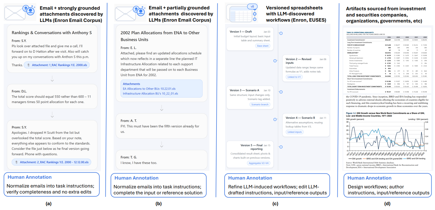
This process yields 172 enterprise-grade workflows—primarily multi-task composite workflows, involving 1,710 spreadsheets and 27 million cells, capturing the intrinsic messy, long-horizon, knowledge-intensive, and collaborative nature of real-world finance & accounting work. 92.4% of workflows involve multiple input and reference sheets, with an average of 8 sheets and a long tail reaching 91 spreadsheets. In this release, we provide full annotations for the 172 workflows, with the evaluation code to be released in a subsequent update.
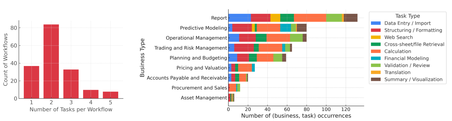
We conduct both human and automated evaluations of frontier AI systems including GPT5.1, Claude Sonnet 4.5, Gemini 3 Pro, Grok 4, and Qwen 3 Max. GPT 5.1 Pro spends 16 mins for each workflow on average and gets the highest pass rate of 38%, while Claude Sonnet 4.5 passes just 25.0%, revealing a substantial performance gap for real-world enterprise scenarios.
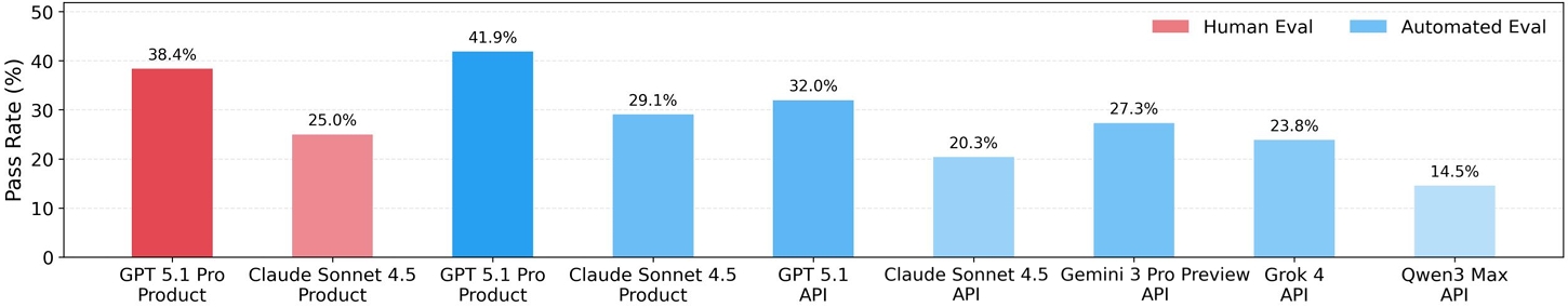
Example 1: Review the Inv & WC Value Adj summary tab and add the missing cross‑sheet data references to the other worksheets so the roll‑up pulls the correct figures. Return the updated file with those links in place.
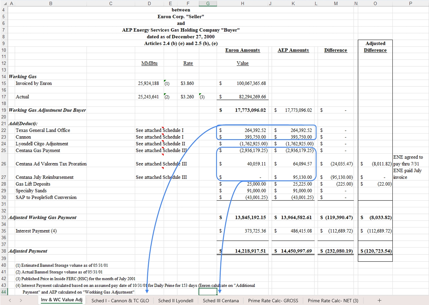
Example 2: Add a new worksheet named "Scenario3" to the same workbook, mirroring the structure, row/column layout, monthly detail table, and chart area of "Scenario1". For Scenario3, update the hedging assumptions to a balanced allocation: 10-Yr 25%, 5-Yr 20%, 1-Yr 15%, May-Sep 20%, Q3 15%. Keep the note "Maximum Monthly Average Short Position to Cover (July Peak) = 30,508 MW" unchanged; only the new sheet should be added, and formulas may be used within it.
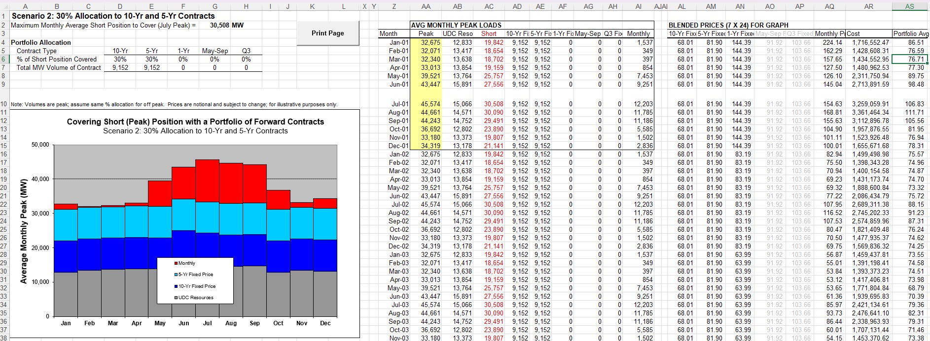
Example 3: Transcribe the content from the image into the Excel file.
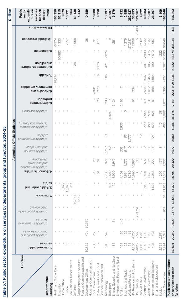
Example 4: Per the red parameters and the Method 1/Method 2 guidance noted in H8 and H9, complete the formulas in columns T and U (starting from1), Note that the starting point for the formulas in columns T and U is 1, representing the initial signal to hold Index 1. In the formulas for columns T and U, 1 represents the signal to hold Index 1, -1 represents the signal to hold Index 2, and 0 represents the signal to make no change. Then complete column I. The method selection in B11 should drive the model so that all cells and charts refresh consistently when switching between methods.
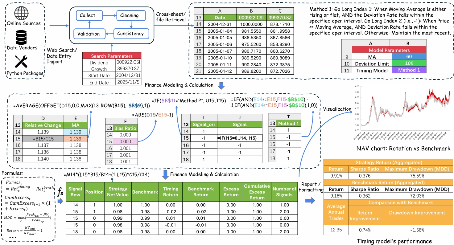
The corpus is released in JSONL format.
Each line corresponds to one workflow-centric example:
{
  "id": "<workflow identifier>",
  "instruction_en": "<English task instruction for a finance & accounting workflow>",
  "source_files": ["<input file name>", "..."],
  "source_files_urls": ["<input file download URL>", "..."],
  "reference_outputs": {
    "files": ["<reference output file name>"],
    "text": "<textual reference output>"
  },
  "reference_file_urls": ["<reference output file download URL>"],
  "task_type": "<task category (e.g., reporting, modeling)>",
  "business_type": "<business domain (e.g., budgeting, trading)>",
  "task_constraints": "<task constraints (e.g., perform modifications rather than generation from scratch)>"
}
Annotations of Finch should NOT appear in training corpora.
If you find any issues with the dataset or have suggestions, please open a discussion in the Community tab — we value your feedback!
@article{dong2025finch,
  title={Finch: Benchmarking Finance \& Accounting across Spreadsheet-Centric Enterprise Workflows},
  author={Dong, Haoyu and Zhang, Pengkun and Gao, Yan and Dong, Xuanyu and Cheng, Yilin and Lu, Mingzhe and Yakefu, Adina and Zheng, Shuxin},
  journal={arXiv preprint arXiv:2512.13168},
  year={2025}
}
📧 Contact: [email protected]