

Uploading and installing conda packages
Anaconda.org is a centralized package repository and distribution platform for the conda ecosystem. The site enables you to both upload your own conda packages and discover conda packages created by other users.
To work with conda packages, you must use the corresponding subdomain `https://conda.anaconda.org`. To install conda packages from the user `travis`, for example, use the repository URL `https://conda.anaconda.org/travis`.Uploading conda packages
This example shows how to build and upload a conda package to Anaconda.org using conda build.
Open Anaconda Prompt (Terminal on macOS/Linux).
If necessary, install the
anaconda-clientandconda-buildpackages by running the following command:conda install anaconda-client conda-buildChoose the repository for which you would like to build the package. In this example, we use a small public conda test package:
# Replace <PACKAGE> with the package name
git clone https://github.com/Anaconda-Platform/anaconda-client
cd anaconda-client/<PACKAGE>/conda/
There are two required files in the example package: meta.yaml and build.sh.
macOS and Linux systems are Unix-like systems. Packages built for Unix-like systems require a
build.shfile, packages built for Windows require abld.batfile, and packages built for both Windows and Unix-like systems require both abuild.shfile and abld.batfile. All packages require ameta.yamlfile.To build the package, turn off automatic Client uploading and then run the
conda buildcommand:conda config --set anaconda_upload no conda build .All packages built using the
You can check where the resulting file was placed by adding the `--output` option:conda buildcommand are placed in a subdirectory of the Anacondaconda-blddirectory.conda build . --outputUpload the test package to Anaconda.org by running the
anaconda uploadcommand:anaconda login # Replace </PATH/TO/PACKAGE_NAME> with the correct file path and package name # Packages can be uploaded with .tar.bz2 or .conda compression formats anaconda upload </PATH/TO/PACKAGE_NAME>.tar.bz2 anaconda upload </PATH/TO/PACKAGE_NAME>.conda
For more information on the .conda format, see Using the .conda compression format.
For more information on conda's overall build framework, see Building conda packages in the official conda docs.
Installing conda packages
You can install conda packages from Anaconda.org by adding channels to your conda configuration.
Public channels
Open Anaconda Prompt (Terminal on macOS/Linux).
Because conda knows how to interact with Anaconda.org, specifying the channel
sean, for example, translates to https://anaconda.org/sean:conda config --add channels seanYou can now install public conda packages from Sean's Anaconda.org account. Try installing the
testcipackage at https://anaconda.org/sean/testci:conda install testci
Private channels
You can install a package from a private channel with a token and a Label:
# Replace <TOKEN> with the provided token
# Replace <CHANNEL> with a user channel
# Replace <LABEL_NAME> with the label name
# Replace <PACKAGE> with the name of the package you want to install
conda install --channel https://conda.anaconda.org/t/<TOKEN>/<CHANNEL>/label/<LABEL_NAME> <PACKAGE>
Tokens are only required if the channel is private.
Finding help for uploading packages
You can obtain a complete list of upload options, including:
- Package channel
- Label
- Availability to other users
- Metadata
To list the options, run the following in Anaconda Prompt (Terminal on macOS/Linux):
anaconda upload -h
Installation
The following sections detail the process for installing and accessing the Anaconda Toolbox Excel add-in. Once installed, get to know your newly added functionality through our Anaconda Toolbox and Anaconda Code documentation.
[Anaconda Code](/tools/excel/code) is included in the Anaconda Toolbox installation.Installing the Anaconda Toolbox Excel add-in
Get started with Anaconda Toolbox instantly:- Open in Excel desktop — requires Excel to be installed on your computer
- Open in Excel online
Company VPNs or firewall settings may affect these links. If you encounter any issues, follow the steps below.
Go to the [Anaconda Toolbox product page on Microsoft AppSource](https://appsource.microsoft.com/en-us/product/office/WA200006518?src=office\&corrid=e512e195-e06f-1a72-091c-b019258ac57c\&omexanonuid=\&referralurl=\&ClientSessionId=222d10cb-7f3d-400b-a75f-0d51b0ba4ab9). Click **Get it now**, then follow the onscreen instructions to open. If necessary, close and reopen Excel for your changes to take effect.Adding the Anaconda Toolbox Excel add-in to your ribbon
From the **Home** tab, click **Add-ins**, then search for *Anaconda*. You should see the **AnacondaToolbox** add-in.<Frame>
<img src="https://mintcdn.com/anaconda-29683c67/IBO7780zo4xe9zAp/images/add_ins.png?fit=max&auto=format&n=IBO7780zo4xe9zAp&q=85&s=c329eea470525b70a3293d1026932921" alt="" data-og-width="1922" width="1922" data-og-height="846" height="846" data-path="images/add_ins.png" data-optimize="true" data-opv="3" srcset="https://mintcdn.com/anaconda-29683c67/IBO7780zo4xe9zAp/images/add_ins.png?w=280&fit=max&auto=format&n=IBO7780zo4xe9zAp&q=85&s=8c21d0b446d249500ac88c0262e21a42 280w, https://mintcdn.com/anaconda-29683c67/IBO7780zo4xe9zAp/images/add_ins.png?w=560&fit=max&auto=format&n=IBO7780zo4xe9zAp&q=85&s=0391cb4c132048d213c3eb12f8988f31 560w, https://mintcdn.com/anaconda-29683c67/IBO7780zo4xe9zAp/images/add_ins.png?w=840&fit=max&auto=format&n=IBO7780zo4xe9zAp&q=85&s=fc759d8506901867b44cf1c5787e1e04 840w, https://mintcdn.com/anaconda-29683c67/IBO7780zo4xe9zAp/images/add_ins.png?w=1100&fit=max&auto=format&n=IBO7780zo4xe9zAp&q=85&s=0d8226d4e68f81efacea8fbcbb84cafb 1100w, https://mintcdn.com/anaconda-29683c67/IBO7780zo4xe9zAp/images/add_ins.png?w=1650&fit=max&auto=format&n=IBO7780zo4xe9zAp&q=85&s=233826a6f1c8144d27363629887f035f 1650w, https://mintcdn.com/anaconda-29683c67/IBO7780zo4xe9zAp/images/add_ins.png?w=2500&fit=max&auto=format&n=IBO7780zo4xe9zAp&q=85&s=d0e3203ebb2a641ec676ab2b63489e98 2500w" />
</Frame>
Launching Anaconda Toolbox
After installing the add-in, go to the **Formulas** tab in Excel's Ribbon. Select **Anaconda Toolbox** to open the Toolbox panel.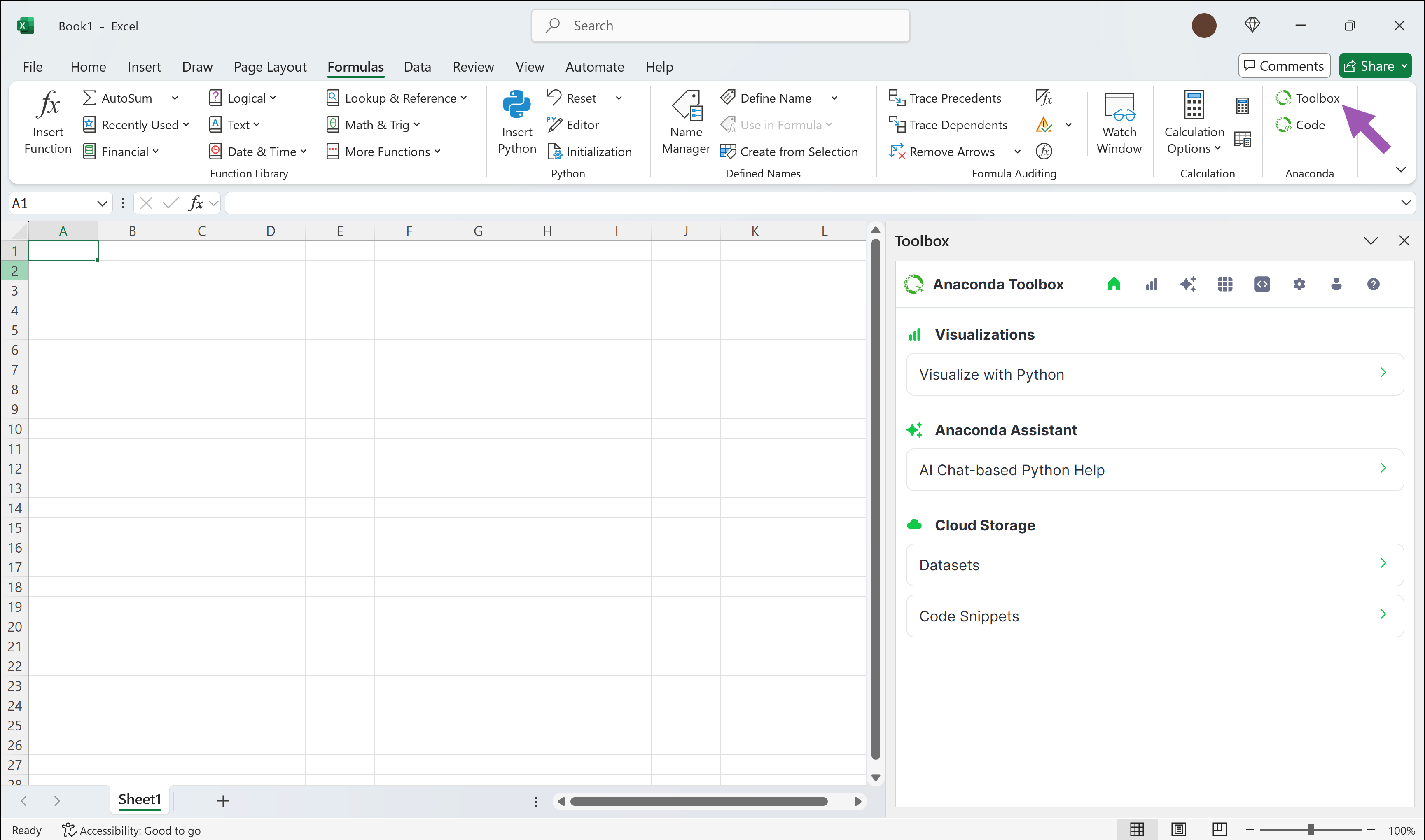
Launching Anaconda Code
After installing the add-in, go to the **Formulas** tab in Excel's Ribbon. Click **Anaconda Code** to open the Code panel.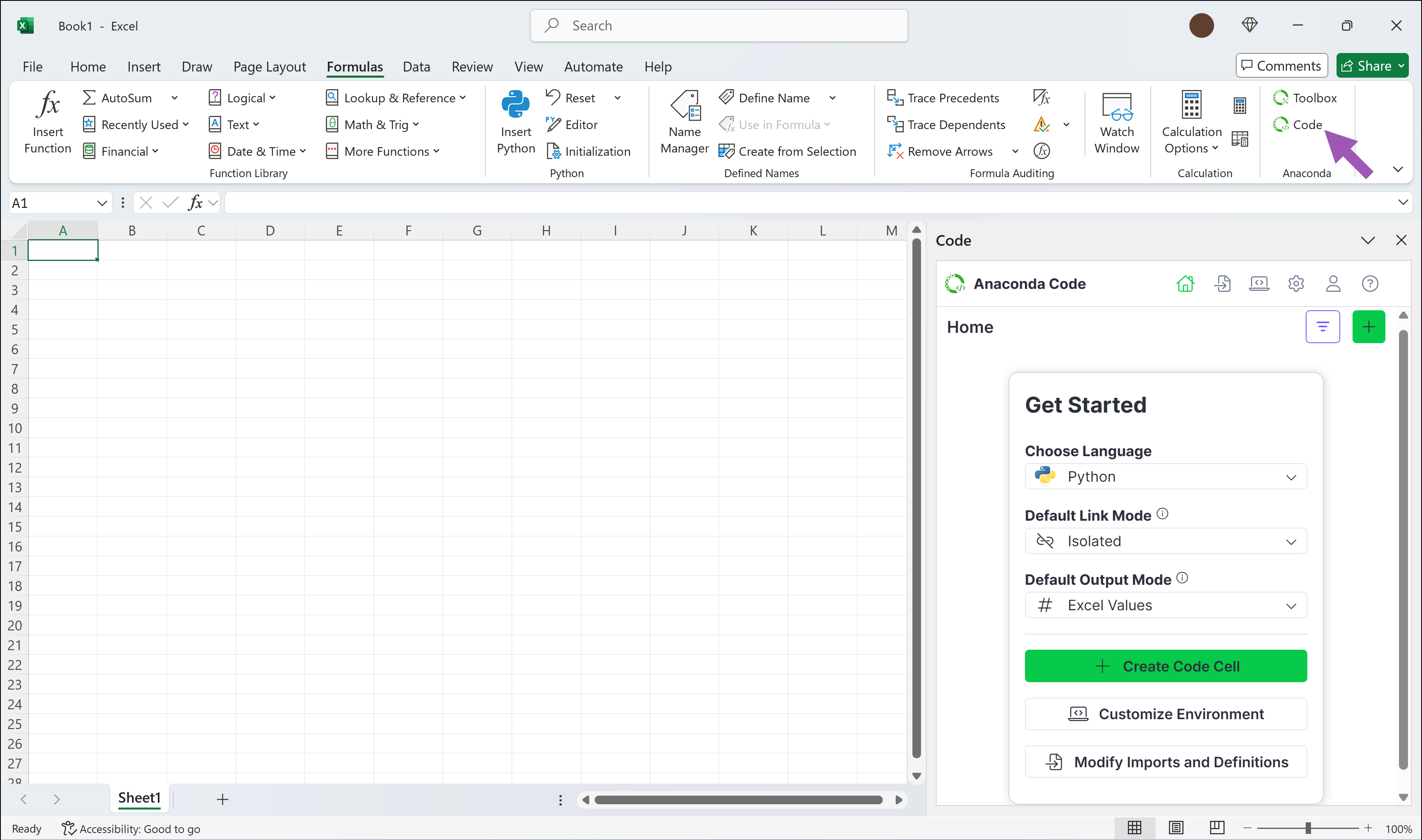
Anaconda Code
export const ExcelRefIcon = () => { return ; };
export const ExcelCellAddressIcon = () => { return ; };
This feature is currently in beta.Anaconda Code empowers you to write Python or R code and run it locally, directly within Excel. This gives you flexibility and control over the environment in your workbook, allowing you to add and remove packages as needed, all while keeping code and data securely within your workbook. Anaconda Code operates independently of Microsoft's Python in Excel feature.
Initializing Anaconda Code
Anaconda Code is included in the [Anaconda Toolbox installation](/tools/excel/install).When you first launch Anaconda Code, you'll be asked to sign in to your Anaconda account.
If you haven't created an Anaconda Code cell yet, you'll be asked to create one.
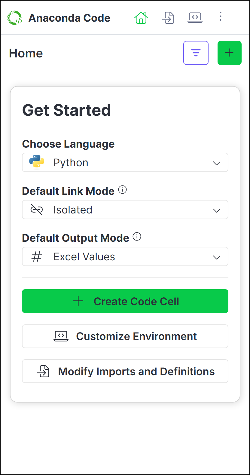
To get started, choose the language for your new Anaconda Code cell, set the default link mode, select the default output mode, and then click Create Code Cell.
Once you've selected a location for your new Anaconda Code cell, use the editor to start writing and running code.
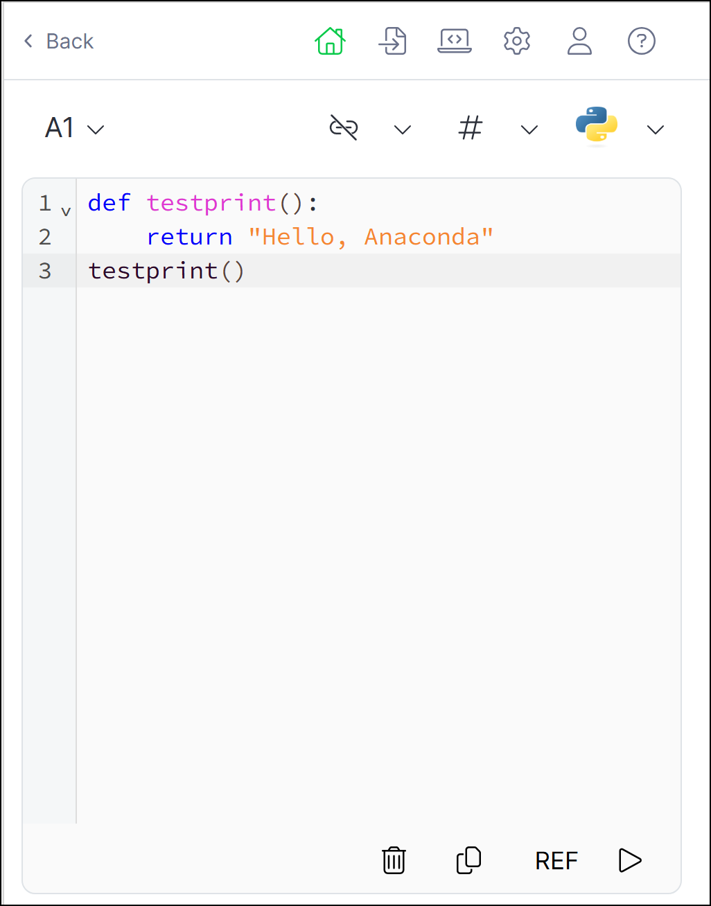
Understanding Anaconda Code
Let's take a look at the different elements within Anaconda Code using the Home tab for reference:
 }>
[Create and run Python or R code](#running-code)
}>
[Create and run Python or R code](#running-code)
<Step title="Imports and Definitions" icon={}> Customize the code that affects all code in your workbook and view script logs
<Step title="Environment" icon={}> Manage the packages and Pyodide or WebR version for your coding environment
<Step title="Settings" icon={}> Modify the default settings for running code
<Step title="Account" icon={}> View profile, subscriptions, sign out, and app details
<Step title="Help" icon={}> Access bug reporting, documentation, community forums, and privacy policy links
<Step title="Active Code Cell Reference" icon={}> The active code cell where your code will run
<Step title="Linking" icon={}> Toggle cell linking between isolated and linked modes
<Step title="Cell Output" icon={}> Choose whether to output cell values as an Excel value or an Anaconda Code object
<Step title="Language" icon={}> Select Python or R for the code cell
<Step title="Delete" icon={}> Delete the code cell
<Step title="Copy" icon={}> Copy the contents of the code editor
<Step title="REF" icon={}> Create a reference to data in the worksheet.
<Step title="Run" icon={}> Run the code in the active code cell
Running code
Create an Anaconda Code cell that can run Python or R code using the following steps:
From Home, click , then select a cell where you want to insert your code.
If you're already in the code editor, select **more** next to the active code cell reference, then **Add New** to create a new code cell. Subsequent code cells will be in the same language as the previously created one. To change the language, first create a new code cell, then change the code cell's language selection in the code editor.Set the cell linking and output options.
Select Python or R as the code language for the cell.
If you change the language for the cell to a language you haven't yet used, you might need to click **Load Environment** to load the new language's environment for the first time.Enter your code in the code editor.
(Optional) If you want to reference a range of data from your spreadsheet or an Anaconda Code object in your code, click REF, then select the range of cells or Anaconda Code cell.
When you use **REF** to select data cells or Anaconda Code cells, Anaconda Code creates a `REF` function in your code that returns a list of lists. The [Imports and Definitions](#customizing-code-initialization) tab includes the following pre-defined functions to help convert the returned list of lists to different data structures. | Function | Use case | Notes | | :---------------------------- | :--------------------------------------------------------------------------------------- | :------------------------------------------------------ | | `to_df(REF())` | Create a [DataFrame](https://pandas.pydata.org/docs/reference/api/pandas.DataFrame.html) | `to_df` assumes your data has headers | | `to_array(REF())` | Create a [NumPy](https://numpy.org/) array | `to_array` assumes all data is of the same type | | `to_list(REF())` | Create a 1D list | `to_list` handles wide (1 x *n*) or tall (*n* x 1) data |You can change the behavior of `to_df()`, `to_array()`, and `to_list()` from the [Imports and Definitions](#customizing-code-initialization) tab. </Tab> <Tab title="R"> | Function | Use case | Notes | | :------------------- | :------------------------------------------------------------------------- | :---------------------------------------------------------------------------------------- | | `to_dataframe()` | Convert to data.frame or tidyverse [tibble](https://tibble.tidyverse.org/) | Converts a list of lists to tabular format, using first row as column names, if available | | `to_matrix()` | Convert to matrix | Converts a list of lists to a matrix structure | | `to_colwise_list()` | Convert to column-wise list of vectors | Transforms row-wise data (list of lists) into column-wise format | | `is_list_of_lists()` | Check data structure | Helper function that verifies if input is properly structured as a list of lists | You can change the behavior of `to_dataframe`, `to_matrix()`, `to_colwise_list()`, and `is_list_of_lists()` from the [Imports and Definitions](#customizing-code-initialization) tab. </Tab>Click Run. The cell will display the return value of the last evaluated expression. Your changes are automatically saved whenever you re-run the code.
If you write code that doesn't have a return value (for example, you define a function but don't call the function) and click **Run**, the cell will display `NoneType`.
Editing code
Do not edit your code in the cell itself; instead, modify and re-run your code directly in Anaconda Code.
An Anaconda.com account is required for users to edit shared code.- From the Home page, click more on the code you want to edit.
- Click Edit in full view to open the edit view.
- Adjust your code, then click Run.
Managing the environment
Anaconda Code hosts a single, self-contained environment, which manages the back-end software packages that enable you to run Python or R code within your Excel workbook. You can manage software packages within this environment to extend your code's processing, visualization, and analytical capabilities, and even select the version of Pyodide (the WASM engine used by PyScript) or WebR (the WASM engine used by WebR) that you want to run.
You can make changes to your environment at any time; however, like with all software projects, altering the environment changes the way the underlying code is interpreted and can cause unintended complications.Choosing a Pyodide or WebR version
The latest version of Pyodide or WebR is used by default for all new spreadsheets. For existing spreadsheets, the Pyodide or WebR versions and packages necessary for your code are pinned to the environment.
You can switch versions using the following steps:
- From the Environment tab, click Edit.
- Select the Pyodide or WebR version.
- Click Save Changes.
Managing software packages
- From the Environment tab, click Edit.
- To add new packages, click Add.
- (Optional for Python) Click the down arrow to add from either PyPI, the PyScript app, or a direct download link to a Python wheel (
.whl). - Search for the package name, then click Add beside the package you want to add.
- Once you've added all the packages you want to include, click Add Packages.
 Packages that contain compiled code might not be compatible with the PyScript or R WASM engine. For more information, visit [PyScript.net](https://pyscript.net/) or [r-wasm.org](https://docs.r-wasm.org/webr/latest/packages.html).
To remove a package, click Edit, then click Delete beside the package you want to remove.
Customizing code initialization
You can think of Anaconda Code's Imports and Definitions as an initialization file for your code or like the first cell in a Jupyter Notebook. All code in this section is available to all cells, whether they are run isolated or linked.
To customize your code's imports:1. On the <Icon icon="file-import" iconType="light" /> **Imports and Definitions** tab, establish the connections to the packages you need to run your code by adding your import statements beneath the `# Add imports` comment.
<Note>
You can only `import` from the packages included in the standard Python or Web R installation and those listed in the **Environment** tab.
</Note>
2. Click **Apply**.
1. From the <Icon icon="file-import" iconType="light" /> **Imports and Definitions** tab, enter any classes or functions you'd like to define beneath the `# Define` comment.

   <Note>
     Anaconda Code comes with pre-defined functions for both Python and R. See [Using the REF function](#using-the-ref-function) to learn more about using these functions.
   </Note>

2. Click **Apply**.

You can now call your definitions in the Anaconda Code editor. To call Python functions directly from a spreadsheet cell, follow the steps in [Creating user-defined functions](#creating-user-defined-functions).
Creating user-defined functions
User-defined functions (UDFs) allow you to write Python or R functions and call them directly from a spreadsheet cell.
**Creating and calling a UDF**1. From the **Imports and Definitions** tab, decorate a function with `@UDF`, as shown in the following example:
```py Python UDF Example theme={null}
@UDF
def my_custom_function(x, y):
return x ** y
```
2. Click **Apply**.
3. In an open cell, enter `=ANACONDA`. If you added the example above to your definitions list, the option to call `ANACONDA.MY_CUSTOM_FUNCTION`
appears in the dropdown.
<Frame>
<img src="https://mintcdn.com/anaconda-29683c67/6fJRxAwYs9izUc34/images/create_udf.png?fit=max&auto=format&n=6fJRxAwYs9izUc34&q=85&s=5572b0cd0c91b1ec16f37833f8da0072" alt="" data-og-width="1704" width="1704" data-og-height="1428" height="1428" data-path="images/create_udf.png" data-optimize="true" data-opv="3" srcset="https://mintcdn.com/anaconda-29683c67/6fJRxAwYs9izUc34/images/create_udf.png?w=280&fit=max&auto=format&n=6fJRxAwYs9izUc34&q=85&s=247d5352f34acb749de8c9f02c18240f 280w, https://mintcdn.com/anaconda-29683c67/6fJRxAwYs9izUc34/images/create_udf.png?w=560&fit=max&auto=format&n=6fJRxAwYs9izUc34&q=85&s=88f9b79bded922be591f1f8c0ab8ba03 560w, https://mintcdn.com/anaconda-29683c67/6fJRxAwYs9izUc34/images/create_udf.png?w=840&fit=max&auto=format&n=6fJRxAwYs9izUc34&q=85&s=066833229713b5d3a64cc6e8037c456c 840w, https://mintcdn.com/anaconda-29683c67/6fJRxAwYs9izUc34/images/create_udf.png?w=1100&fit=max&auto=format&n=6fJRxAwYs9izUc34&q=85&s=fa27c4109d98adf81c92b28f554e5f86 1100w, https://mintcdn.com/anaconda-29683c67/6fJRxAwYs9izUc34/images/create_udf.png?w=1650&fit=max&auto=format&n=6fJRxAwYs9izUc34&q=85&s=9b6d9cd3ee1b3d56255efe1bddc9a93e 1650w, https://mintcdn.com/anaconda-29683c67/6fJRxAwYs9izUc34/images/create_udf.png?w=2500&fit=max&auto=format&n=6fJRxAwYs9izUc34&q=85&s=74d66126646824dc6fc053a42fb8d0fe 2500w" />
</Frame>
4. Arrow down to `ANACONDA.MY_CUSTOM_FUNCTION`, press Tab, and then complete the function.
5. Use Ctrl+Enter (Windows)/Ctrl+Return (macOS) to run the code.
<Tip>
If you'd prefer the UDF uses a name other than the function name, use the `name` argument to provide a unique name. Set `nested` to False to remove `ANACONDA.` from the name.
```py Renaming Python UDF Example theme={null}
@UDF(name="MYBANK.PORTFOLIO_ANALYSIS", nested=False)
def my_custom_function(x, y):
return x ** y
```
<Frame>
<img src="https://mintcdn.com/anaconda-29683c67/6fJRxAwYs9izUc34/images/create_udf_custom_name.png?fit=max&auto=format&n=6fJRxAwYs9izUc34&q=85&s=373fe4433136ca79c235ad8ca82c2f75" alt="" data-og-width="1698" width="1698" data-og-height="1428" height="1428" data-path="images/create_udf_custom_name.png" data-optimize="true" data-opv="3" srcset="https://mintcdn.com/anaconda-29683c67/6fJRxAwYs9izUc34/images/create_udf_custom_name.png?w=280&fit=max&auto=format&n=6fJRxAwYs9izUc34&q=85&s=0c732829a891824eef2bcd3f1765180d 280w, https://mintcdn.com/anaconda-29683c67/6fJRxAwYs9izUc34/images/create_udf_custom_name.png?w=560&fit=max&auto=format&n=6fJRxAwYs9izUc34&q=85&s=851c16b280782e58675068d8a9f342da 560w, https://mintcdn.com/anaconda-29683c67/6fJRxAwYs9izUc34/images/create_udf_custom_name.png?w=840&fit=max&auto=format&n=6fJRxAwYs9izUc34&q=85&s=7d19999c27fc6440d58bebe0beb2e9f6 840w, https://mintcdn.com/anaconda-29683c67/6fJRxAwYs9izUc34/images/create_udf_custom_name.png?w=1100&fit=max&auto=format&n=6fJRxAwYs9izUc34&q=85&s=b69b4fbbc3433f8bc6d85748128a4d7d 1100w, https://mintcdn.com/anaconda-29683c67/6fJRxAwYs9izUc34/images/create_udf_custom_name.png?w=1650&fit=max&auto=format&n=6fJRxAwYs9izUc34&q=85&s=1fcda28ebc077cb9b82a3cc61e397369 1650w, https://mintcdn.com/anaconda-29683c67/6fJRxAwYs9izUc34/images/create_udf_custom_name.png?w=2500&fit=max&auto=format&n=6fJRxAwYs9izUc34&q=85&s=701b6b1bb35d0ed9a4458461534c76e4 2500w" />
</Frame>
</Tip>
**Using range arguments**
Specifying a `UDF.Range` argument tells Excel that the input of the function is a 2D range. Without specifying this, Excel will show a `#CALC! Unliftable Array` error if a 2D range is passed into the UDF. Parameters specified as `UDF.Range` will always be passed as a 2D array to the function, even if a single cell is passed in.
Example usage of `UDF.Range`:
```py Python Range Example theme={null}
@UDF
def square_me(data: UDF.Range) -> UDF.Range:
return [[val ** 2 for val in row] for row in data]
```
You can also add type hints for ranges. For example,`UDF.Range[str]`.
1. From the **Imports and Definitions** tab, register the UDF with `UDF.register()` and pass the function as an argument, as shown in the following example:

   <Note>
     The UDF must be registered after the function is defined.
   </Note>

   ```r R UDF Example theme={null}
   my_custom_r_function <- function(x, y) {
       x ^ y
   }
   UDF.register(my_custom_r_function)
   ```

2. Click **Save and Apply**.

3. In an open cell, enter `=ANACONDA`. If you added the example above to your definitions list, the option to call `ANACONDA.MY_CUSTOM_R_FUNCTION`
   appears in the dropdown.

   <Frame>
     <img src="https://mintcdn.com/anaconda-29683c67/6fJRxAwYs9izUc34/images/create_udf_r.png?fit=max&auto=format&n=6fJRxAwYs9izUc34&q=85&s=010bdb18a5ff8d5bc2bc38940eb0e120" alt="" data-og-width="1734" width="1734" data-og-height="1716" height="1716" data-path="images/create_udf_r.png" data-optimize="true" data-opv="3" srcset="https://mintcdn.com/anaconda-29683c67/6fJRxAwYs9izUc34/images/create_udf_r.png?w=280&fit=max&auto=format&n=6fJRxAwYs9izUc34&q=85&s=1239e88fdc6a9cfa062897f742b8bc1c 280w, https://mintcdn.com/anaconda-29683c67/6fJRxAwYs9izUc34/images/create_udf_r.png?w=560&fit=max&auto=format&n=6fJRxAwYs9izUc34&q=85&s=ffb973876271c5c2f50b60b61b7bb4c2 560w, https://mintcdn.com/anaconda-29683c67/6fJRxAwYs9izUc34/images/create_udf_r.png?w=840&fit=max&auto=format&n=6fJRxAwYs9izUc34&q=85&s=332b09f3ae0ff6e2942ea545ef03ca2a 840w, https://mintcdn.com/anaconda-29683c67/6fJRxAwYs9izUc34/images/create_udf_r.png?w=1100&fit=max&auto=format&n=6fJRxAwYs9izUc34&q=85&s=0348520653693a4a1ca82e8f6b4ebc29 1100w, https://mintcdn.com/anaconda-29683c67/6fJRxAwYs9izUc34/images/create_udf_r.png?w=1650&fit=max&auto=format&n=6fJRxAwYs9izUc34&q=85&s=74a2709a286a9b5afadd15175432749d 1650w, https://mintcdn.com/anaconda-29683c67/6fJRxAwYs9izUc34/images/create_udf_r.png?w=2500&fit=max&auto=format&n=6fJRxAwYs9izUc34&q=85&s=fa64c6ee67a4c6f4e081990aa68b4ad1 2500w" />
   </Frame>

4. Arrow down to `ANACONDA.MY_CUSTOM_R_FUNCTION`, press Tab, and then complete the function call.

5. Use Ctrl+Enter (Windows)/Ctrl+Return (macOS) to run the code.

<Tip>
  If you'd prefer the UDF uses a name other than the function name, register the function with the UDF, then use the `name` argument to provide a unique name and set `nested` to False to remove `ANACONDA.` from the name.

  ```r Renaming R UDF Example theme={null}
  my_custom_r_function <- function(x, y) {
      x ^ y
  }
  UDF.register(my_custom_r_function, name="MYBANK.PORTFOLIO_ANALYSIS", nested=FALSE)
  ```

  <Frame>
    <img src="https://mintcdn.com/anaconda-29683c67/6fJRxAwYs9izUc34/images/create_udf_r_custom_name.png?fit=max&auto=format&n=6fJRxAwYs9izUc34&q=85&s=bbe57a6e5a269a3291421899cbbb5654" alt="" data-og-width="1694" width="1694" data-og-height="1712" height="1712" data-path="images/create_udf_r_custom_name.png" data-optimize="true" data-opv="3" srcset="https://mintcdn.com/anaconda-29683c67/6fJRxAwYs9izUc34/images/create_udf_r_custom_name.png?w=280&fit=max&auto=format&n=6fJRxAwYs9izUc34&q=85&s=1c8cb2c1c1ad3a50d61d5bbddff9e482 280w, https://mintcdn.com/anaconda-29683c67/6fJRxAwYs9izUc34/images/create_udf_r_custom_name.png?w=560&fit=max&auto=format&n=6fJRxAwYs9izUc34&q=85&s=69b44583db7858fb51aef174c9687e2d 560w, https://mintcdn.com/anaconda-29683c67/6fJRxAwYs9izUc34/images/create_udf_r_custom_name.png?w=840&fit=max&auto=format&n=6fJRxAwYs9izUc34&q=85&s=e64878144f327129b4cfb363cf60f712 840w, https://mintcdn.com/anaconda-29683c67/6fJRxAwYs9izUc34/images/create_udf_r_custom_name.png?w=1100&fit=max&auto=format&n=6fJRxAwYs9izUc34&q=85&s=5a7203d44ecffc992850bdce56bd0fb0 1100w, https://mintcdn.com/anaconda-29683c67/6fJRxAwYs9izUc34/images/create_udf_r_custom_name.png?w=1650&fit=max&auto=format&n=6fJRxAwYs9izUc34&q=85&s=13195fc72350cd26e725307f3a8e8ff7 1650w, https://mintcdn.com/anaconda-29683c67/6fJRxAwYs9izUc34/images/create_udf_r_custom_name.png?w=2500&fit=max&auto=format&n=6fJRxAwYs9izUc34&q=85&s=2848fabfdc2a327fbe4a6262354cc776 2500w" />
  </Frame>
</Tip>

**Using range arguments**

Setting the `range_args` parameter tells Excel that the input of the function is a 2D range.  Without specifying this, Excel will show a `#CALC! Unliftable Array` error if a 2D range is passed into the UDF. Parameters specified as `range_args` will always be passed as a 2D array to the function, even if a single cell is passed in.

Example usage of `range_args`:

```r R Range Example theme={null}
my_custom_r_function <- function(data) {
    sum(data)
}
UDF.register(my_custom_r_function, range_args=c("data"))
```

**Adding function documentation**

To add documentation to your function, use the `doc` parameter:

```r R Documentation Example theme={null}
my_custom_r_function <- function(x, y) {
    x ^ y
}
UDF.register(my_custom_r_function, doc="Computes x raised to the power of y.")
```
Modifying workbook settings
While you can adjust the settings for running code in your workbook on a case-by-case basis when creating and editing code, you can also assign default settings from the Settings tab.
Cell linking
When a code cell is run in **isolated** mode, its code runs independently of other cells. Variables defined within an isolated code cell can't be referenced by other code cells, and variables in other code cells likewise can't be referenced by the isolated code cell.<Frame>
<img src="https://mintcdn.com/anaconda-29683c67/9H-5W4tTlP7-Fn32/images/cell_isolated_mode.png?fit=max&auto=format&n=9H-5W4tTlP7-Fn32&q=85&s=e28a4ac7b0c21c11b11f4947f303d02c" alt="Two code cells in isolated mode where the second cell cannot access variables from the first" data-og-width="1684" width="1684" data-og-height="948" height="948" data-path="images/cell_isolated_mode.png" data-optimize="true" data-opv="3" srcset="https://mintcdn.com/anaconda-29683c67/9H-5W4tTlP7-Fn32/images/cell_isolated_mode.png?w=280&fit=max&auto=format&n=9H-5W4tTlP7-Fn32&q=85&s=cc926655d310e577b8d716461bab68a6 280w, https://mintcdn.com/anaconda-29683c67/9H-5W4tTlP7-Fn32/images/cell_isolated_mode.png?w=560&fit=max&auto=format&n=9H-5W4tTlP7-Fn32&q=85&s=7d8061a23efbb3d233fde9e387c98420 560w, https://mintcdn.com/anaconda-29683c67/9H-5W4tTlP7-Fn32/images/cell_isolated_mode.png?w=840&fit=max&auto=format&n=9H-5W4tTlP7-Fn32&q=85&s=bf8d89742812a7cbca0caeca37f2562b 840w, https://mintcdn.com/anaconda-29683c67/9H-5W4tTlP7-Fn32/images/cell_isolated_mode.png?w=1100&fit=max&auto=format&n=9H-5W4tTlP7-Fn32&q=85&s=2b3785789f9b826b69fe4b6e32e3a76a 1100w, https://mintcdn.com/anaconda-29683c67/9H-5W4tTlP7-Fn32/images/cell_isolated_mode.png?w=1650&fit=max&auto=format&n=9H-5W4tTlP7-Fn32&q=85&s=b552bbb1e33607ce2b90415a01e889ee 1650w, https://mintcdn.com/anaconda-29683c67/9H-5W4tTlP7-Fn32/images/cell_isolated_mode.png?w=2500&fit=max&auto=format&n=9H-5W4tTlP7-Fn32&q=85&s=75b04f2cbcbd411a62405774e632172d 2500w" />
</Frame>
In the above image, the `output_of_B2` variable is defined in cell B2 and assigned the string `"I'm the B2 cell!"`. When this code is run in the B2 code cell, the B2 cell displays `"I'm the B2 cell!"`. However, since both cells are running in isolated mode, when `output_of_B2` is referenced in the B4 code cell, the B4 cell displays a `#VALUE!` error because B4 cannot access the variable in B2.
**Using the `REF` function**
You can bypass isolation rules as needed using the `REF` function to create a reference from one isolated code cell to another.
<Frame>
<img src="https://mintcdn.com/anaconda-29683c67/QCWY8EsGZWJYinOU/images/isolated_ref_cell.png?fit=max&auto=format&n=QCWY8EsGZWJYinOU&q=85&s=0a6287dd90c0c73498e23d6557133461" alt="A code cell using the REF function to reference another cell's output" data-og-width="1704" width="1704" data-og-height="962" height="962" data-path="images/isolated_ref_cell.png" data-optimize="true" data-opv="3" srcset="https://mintcdn.com/anaconda-29683c67/QCWY8EsGZWJYinOU/images/isolated_ref_cell.png?w=280&fit=max&auto=format&n=QCWY8EsGZWJYinOU&q=85&s=b56a71f44090f7a49c6cd2fa07fed96b 280w, https://mintcdn.com/anaconda-29683c67/QCWY8EsGZWJYinOU/images/isolated_ref_cell.png?w=560&fit=max&auto=format&n=QCWY8EsGZWJYinOU&q=85&s=966d9ab29e616226cd6c3eeca069b4d9 560w, https://mintcdn.com/anaconda-29683c67/QCWY8EsGZWJYinOU/images/isolated_ref_cell.png?w=840&fit=max&auto=format&n=QCWY8EsGZWJYinOU&q=85&s=78a913f30c04c90f1e3c5f2653d60824 840w, https://mintcdn.com/anaconda-29683c67/QCWY8EsGZWJYinOU/images/isolated_ref_cell.png?w=1100&fit=max&auto=format&n=QCWY8EsGZWJYinOU&q=85&s=68fed1efc9937f1bbe78c4c4dd9b25c6 1100w, https://mintcdn.com/anaconda-29683c67/QCWY8EsGZWJYinOU/images/isolated_ref_cell.png?w=1650&fit=max&auto=format&n=QCWY8EsGZWJYinOU&q=85&s=73d17eaa5428cff9c8aa85b61a8f937b 1650w, https://mintcdn.com/anaconda-29683c67/QCWY8EsGZWJYinOU/images/isolated_ref_cell.png?w=2500&fit=max&auto=format&n=QCWY8EsGZWJYinOU&q=85&s=21f7f82c541d536e9dd555243fd1ed02 2500w" />
</Frame>
In the above image, the B4 cell now includes a reference to the B2 cell, `REF("B2")`. When the B4 code cell is run, it returns the value of B2, `"I'm the B2 cell!"`. Changes to the B4 cell don't cause the B2 cell to recalculate, but changes to the B2 cell will cause the B4 cell to recalculate. Code cells can include multiple `REF` function references, and changes to any referenced cells (in this example, B2) will cause the referencing cells to recalculate (in this example, B4).
**Working with code objects**
If you reference a cell that's set to output a code object, the `REF` function will return an instance of that object in the referencing cell.
<Frame>
<img src="https://mintcdn.com/anaconda-29683c67/6fJRxAwYs9izUc34/images/code_object_isolated.png?fit=max&auto=format&n=6fJRxAwYs9izUc34&q=85&s=a88c0a285d085c14ab3c12afe5120cb8" alt="A code cell referencing another cell that outputs a list object" data-og-width="1718" width="1718" data-og-height="968" height="968" data-path="images/code_object_isolated.png" data-optimize="true" data-opv="3" srcset="https://mintcdn.com/anaconda-29683c67/6fJRxAwYs9izUc34/images/code_object_isolated.png?w=280&fit=max&auto=format&n=6fJRxAwYs9izUc34&q=85&s=9701200f23ffc2a1393da4012ea21c45 280w, https://mintcdn.com/anaconda-29683c67/6fJRxAwYs9izUc34/images/code_object_isolated.png?w=560&fit=max&auto=format&n=6fJRxAwYs9izUc34&q=85&s=33680dd70b91eb2c9cbe4fddbd252bf7 560w, https://mintcdn.com/anaconda-29683c67/6fJRxAwYs9izUc34/images/code_object_isolated.png?w=840&fit=max&auto=format&n=6fJRxAwYs9izUc34&q=85&s=e99f2aff1f205424347212780948291c 840w, https://mintcdn.com/anaconda-29683c67/6fJRxAwYs9izUc34/images/code_object_isolated.png?w=1100&fit=max&auto=format&n=6fJRxAwYs9izUc34&q=85&s=ad5325ba43d4a75b05fbe424db54083c 1100w, https://mintcdn.com/anaconda-29683c67/6fJRxAwYs9izUc34/images/code_object_isolated.png?w=1650&fit=max&auto=format&n=6fJRxAwYs9izUc34&q=85&s=addd1a2ae6323b3829d2ced2df6235dc 1650w, https://mintcdn.com/anaconda-29683c67/6fJRxAwYs9izUc34/images/code_object_isolated.png?w=2500&fit=max&auto=format&n=6fJRxAwYs9izUc34&q=85&s=4d31cd9b92a61ba53043b2ad2e460514 2500w" />
</Frame>
In the above image, the B2 code cell is set to output a code object (in this case, a list). Because the output of B2 is a <Tooltip tip="A non-scalar value is a data structure that contains multiple values, such as a list, dictionary, or tuple.">non-scalar value</Tooltip>, we see `</> list` in B2. In the B4 code cell, we define a variable called `output_of_B2` and assign a `REF` function that references cell B2. The output mode for the B4 code cell is set to "Excel Values", so the list spills across multiple cells in the spreadsheet.
**Benefits of isolated mode**
The benefit of using the isolated mode is that referenced cells are not recalculated when changes are made to referencing cells. For complex processes, this allows you to:
* separate code that doesn't change frequently from code you modify often.
* reduce unnecessary recalculations of computationally intensive operations.
* create a more modular approach to your data analysis.
* improve performance when working with larger datasets.
<Frame>
  <img src="https://mintcdn.com/anaconda-29683c67/9H-5W4tTlP7-Fn32/images/cell_linked_mode.png?fit=max&auto=format&n=9H-5W4tTlP7-Fn32&q=85&s=e4be8b9c4344868b197fef9062b442b6" alt="" data-og-width="1698" width="1698" data-og-height="952" height="952" data-path="images/cell_linked_mode.png" data-optimize="true" data-opv="3" srcset="https://mintcdn.com/anaconda-29683c67/9H-5W4tTlP7-Fn32/images/cell_linked_mode.png?w=280&fit=max&auto=format&n=9H-5W4tTlP7-Fn32&q=85&s=3d8e440d25369edf953f0400a37991c8 280w, https://mintcdn.com/anaconda-29683c67/9H-5W4tTlP7-Fn32/images/cell_linked_mode.png?w=560&fit=max&auto=format&n=9H-5W4tTlP7-Fn32&q=85&s=e52b875cdd5cabe82921e39e94cdb9bf 560w, https://mintcdn.com/anaconda-29683c67/9H-5W4tTlP7-Fn32/images/cell_linked_mode.png?w=840&fit=max&auto=format&n=9H-5W4tTlP7-Fn32&q=85&s=4c5f84e2322fb3ea57ef0a60e76c0053 840w, https://mintcdn.com/anaconda-29683c67/9H-5W4tTlP7-Fn32/images/cell_linked_mode.png?w=1100&fit=max&auto=format&n=9H-5W4tTlP7-Fn32&q=85&s=be2fc5900b83edc477e12dd6c17c6c1b 1100w, https://mintcdn.com/anaconda-29683c67/9H-5W4tTlP7-Fn32/images/cell_linked_mode.png?w=1650&fit=max&auto=format&n=9H-5W4tTlP7-Fn32&q=85&s=785ebaa8887db14cc357ee7716cc60be 1650w, https://mintcdn.com/anaconda-29683c67/9H-5W4tTlP7-Fn32/images/cell_linked_mode.png?w=2500&fit=max&auto=format&n=9H-5W4tTlP7-Fn32&q=85&s=29443653e2dcf1186f59fbccf9a50790 2500w" />
</Frame>

In the above image, both the B2 and B4 cell are running in linked mode. The `output_of_B2` variable is defined in cell B2 and assigned the string `"I'm the B2 cell!"`. When this code is run in the B2 code cell, the B2 cell displays `"I'm the B2 cell!"`. The `output_of_B2` variable is then referenced in the B4 code cell, causing the B4 cell to also display `"I'm the B2 cell!"`.

**Benefits of linked mode**

Linked mode is useful when:

* you want to create a continuous workflow across multiple cells.
* you need to share variables and objects between different parts of your analysis.
* your code follows a linear execution path.
Cell output
| Output | Description |
|---|---|
| Excel Values | When outputting a DataFrame, array, list, and so on, the values will "spill" to fill the required space. If the spill were to overwrite cells containing data, the cell displays a #SPILL error. |
| Local Code Object | For certain object types, you can view the contents in a "Card View" by clicking the cell. You can reference this cell and the returned object like you would any other object. |
Troubleshooting
If you encounter an issue that is not listed here, you can obtain support for Anaconda through the Anaconda community forums or by opening a support ticket.
Error installing functions
This error can occur when Excel loads the Anaconda Toolbox add-in and registers its custom functions. This error happens within Excel and cannot be resolved by the Anaconda Toolbox. Close and reopen Excel. If the issue persists, uninstall the Anaconda Toolbox add-in, then reinstall.Anaconda Code
export const ExcelRefIcon = () => { return ; };
export const ExcelCellAddressIcon = () => { return ; };
This feature is currently in beta.Anaconda Code empowers you to write Python or R code and run it locally, directly within Excel. This gives you flexibility and control over the environment in your workbook, allowing you to add and remove packages as needed, all while keeping code and data securely within your workbook. Anaconda Code operates independently of Microsoft's Python in Excel feature.
Initializing Anaconda Code
Anaconda Code is included in the [Anaconda Toolbox installation](/tools/excel/install).When you first launch Anaconda Code, you'll be asked to sign in to your Anaconda account.
If you haven't created an Anaconda Code cell yet, you'll be asked to create one.
To get started, choose the language for your new Anaconda Code cell, set the default link mode, select the default output mode, and then click Create Code Cell.
Once you've selected a location for your new Anaconda Code cell, use the editor to start writing and running code.
Understanding Anaconda Code
Let's take a look at the different elements within Anaconda Code using the Home tab for reference:
}>
[Create and run Python or R code](#running-code)
<Step title="Imports and Definitions" icon={}> Customize the code that affects all code in your workbook and view script logs
<Step title="Environment" icon={}> Manage the packages and Pyodide or WebR version for your coding environment
<Step title="Settings" icon={}> Modify the default settings for running code
<Step title="Account" icon={}> View profile, subscriptions, sign out, and app details
<Step title="Help" icon={}> Access bug reporting, documentation, community forums, and privacy policy links
<Step title="Active Code Cell Reference" icon={}> The active code cell where your code will run
<Step title="Linking" icon={}> Toggle cell linking between isolated and linked modes
<Step title="Cell Output" icon={}> Choose whether to output cell values as an Excel value or an Anaconda Code object
<Step title="Language" icon={}> Select Python or R for the code cell
<Step title="Delete" icon={}> Delete the code cell
<Step title="Copy" icon={}> Copy the contents of the code editor
<Step title="REF" icon={}> Create a reference to data in the worksheet.
<Step title="Run" icon={}> Run the code in the active code cell
Running code
Create an Anaconda Code cell that can run Python or R code using the following steps:
From Home, click , then select a cell where you want to insert your code.
If you're already in the code editor, select **more** next to the active code cell reference, then **Add New** to create a new code cell. Subsequent code cells will be in the same language as the previously created one. To change the language, first create a new code cell, then change the code cell's language selection in the code editor.Set the cell linking and output options.
Select Python or R as the code language for the cell.
If you change the language for the cell to a language you haven't yet used, you might need to click **Load Environment** to load the new language's environment for the first time.Enter your code in the code editor.
(Optional) If you want to reference a range of data from your spreadsheet or an Anaconda Code object in your code, click REF, then select the range of cells or Anaconda Code cell.
When you use **REF** to select data cells or Anaconda Code cells, Anaconda Code creates a `REF` function in your code that returns a list of lists. The [Imports and Definitions](#customizing-code-initialization) tab includes the following pre-defined functions to help convert the returned list of lists to different data structures. | Function | Use case | Notes | | :---------------------------- | :--------------------------------------------------------------------------------------- | :------------------------------------------------------ | | `to_df(REF())` | Create a [DataFrame](https://pandas.pydata.org/docs/reference/api/pandas.DataFrame.html) | `to_df` assumes your data has headers | | `to_array(REF())` | Create a [NumPy](https://numpy.org/) array | `to_array` assumes all data is of the same type | | `to_list(REF())` | Create a 1D list | `to_list` handles wide (1 x *n*) or tall (*n* x 1) data |You can change the behavior of `to_df()`, `to_array()`, and `to_list()` from the [Imports and Definitions](#customizing-code-initialization) tab. </Tab> <Tab title="R"> | Function | Use case | Notes | | :------------------- | :------------------------------------------------------------------------- | :---------------------------------------------------------------------------------------- | | `to_dataframe()` | Convert to data.frame or tidyverse [tibble](https://tibble.tidyverse.org/) | Converts a list of lists to tabular format, using first row as column names, if available | | `to_matrix()` | Convert to matrix | Converts a list of lists to a matrix structure | | `to_colwise_list()` | Convert to column-wise list of vectors | Transforms row-wise data (list of lists) into column-wise format | | `is_list_of_lists()` | Check data structure | Helper function that verifies if input is properly structured as a list of lists | You can change the behavior of `to_dataframe`, `to_matrix()`, `to_colwise_list()`, and `is_list_of_lists()` from the [Imports and Definitions](#customizing-code-initialization) tab. </Tab>Click Run. The cell will display the return value of the last evaluated expression. Your changes are automatically saved whenever you re-run the code.
If you write code that doesn't have a return value (for example, you define a function but don't call the function) and click **Run**, the cell will display `NoneType`.
Editing code
Do not edit your code in the cell itself; instead, modify and re-run your code directly in Anaconda Code.
An Anaconda.com account is required for users to edit shared code.- From the Home page, click more on the code you want to edit.
- Click Edit in full view to open the edit view.
- Adjust your code, then click Run.
Managing the environment
Anaconda Code hosts a single, self-contained environment, which manages the back-end software packages that enable you to run Python or R code within your Excel workbook. You can manage software packages within this environment to extend your code's processing, visualization, and analytical capabilities, and even select the version of Pyodide (the WASM engine used by PyScript) or WebR (the WASM engine used by WebR) that you want to run.
You can make changes to your environment at any time; however, like with all software projects, altering the environment changes the way the underlying code is interpreted and can cause unintended complications.Choosing a Pyodide or WebR version
The latest version of Pyodide or WebR is used by default for all new spreadsheets. For existing spreadsheets, the Pyodide or WebR versions and packages necessary for your code are pinned to the environment.
You can switch versions using the following steps:
- From the Environment tab, click Edit.
- Select the Pyodide or WebR version.
- Click Save Changes.
Managing software packages
- From the Environment tab, click Edit.
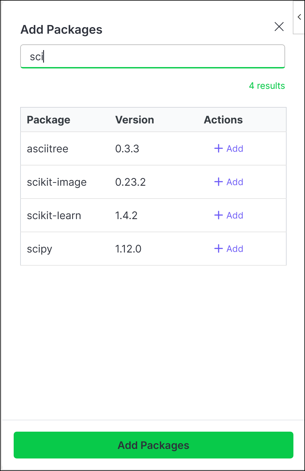
- To add new packages, click Add.
- (Optional for Python) Click the down arrow to add from either PyPI, the PyScript app, or a direct download link to a Python wheel (
.whl). - Search for the package name, then click Add beside the package you want to add.
- Once you've added all the packages you want to include, click Add Packages.
Packages that contain compiled code might not be compatible with the PyScript or R WASM engine. For more information, visit [PyScript.net](https://pyscript.net/) or [r-wasm.org](https://docs.r-wasm.org/webr/latest/packages.html).
To remove a package, click Edit, then click Delete beside the package you want to remove.
Customizing code initialization
You can think of Anaconda Code's Imports and Definitions as an initialization file for your code or like the first cell in a Jupyter Notebook. All code in this section is available to all cells, whether they are run isolated or linked.
To customize your code's imports:1. On the <Icon icon="file-import" iconType="light" /> **Imports and Definitions** tab, establish the connections to the packages you need to run your code by adding your import statements beneath the `# Add imports` comment.
<Note>
You can only `import` from the packages included in the standard Python or Web R installation and those listed in the **Environment** tab.
</Note>
2. Click **Apply**.
1. From the <Icon icon="file-import" iconType="light" /> **Imports and Definitions** tab, enter any classes or functions you'd like to define beneath the `# Define` comment.

   <Note>
     Anaconda Code comes with pre-defined functions for both Python and R. See [Using the REF function](#using-the-ref-function) to learn more about using these functions.
   </Note>

2. Click **Apply**.

You can now call your definitions in the Anaconda Code editor. To call Python functions directly from a spreadsheet cell, follow the steps in [Creating user-defined functions](#creating-user-defined-functions).
Creating user-defined functions
User-defined functions (UDFs) allow you to write Python or R functions and call them directly from a spreadsheet cell.
**Creating and calling a UDF**1. From the **Imports and Definitions** tab, decorate a function with `@UDF`, as shown in the following example:
```py Python UDF Example theme={null}
@UDF
def my_custom_function(x, y):
return x ** y
```
2. Click **Apply**.
3. In an open cell, enter `=ANACONDA`. If you added the example above to your definitions list, the option to call `ANACONDA.MY_CUSTOM_FUNCTION`
appears in the dropdown.
<Frame>
<img src="https://mintcdn.com/anaconda-29683c67/6fJRxAwYs9izUc34/images/create_udf.png?fit=max&auto=format&n=6fJRxAwYs9izUc34&q=85&s=5572b0cd0c91b1ec16f37833f8da0072" alt="" data-og-width="1704" width="1704" data-og-height="1428" height="1428" data-path="images/create_udf.png" data-optimize="true" data-opv="3" srcset="https://mintcdn.com/anaconda-29683c67/6fJRxAwYs9izUc34/images/create_udf.png?w=280&fit=max&auto=format&n=6fJRxAwYs9izUc34&q=85&s=247d5352f34acb749de8c9f02c18240f 280w, https://mintcdn.com/anaconda-29683c67/6fJRxAwYs9izUc34/images/create_udf.png?w=560&fit=max&auto=format&n=6fJRxAwYs9izUc34&q=85&s=88f9b79bded922be591f1f8c0ab8ba03 560w, https://mintcdn.com/anaconda-29683c67/6fJRxAwYs9izUc34/images/create_udf.png?w=840&fit=max&auto=format&n=6fJRxAwYs9izUc34&q=85&s=066833229713b5d3a64cc6e8037c456c 840w, https://mintcdn.com/anaconda-29683c67/6fJRxAwYs9izUc34/images/create_udf.png?w=1100&fit=max&auto=format&n=6fJRxAwYs9izUc34&q=85&s=fa27c4109d98adf81c92b28f554e5f86 1100w, https://mintcdn.com/anaconda-29683c67/6fJRxAwYs9izUc34/images/create_udf.png?w=1650&fit=max&auto=format&n=6fJRxAwYs9izUc34&q=85&s=9b6d9cd3ee1b3d56255efe1bddc9a93e 1650w, https://mintcdn.com/anaconda-29683c67/6fJRxAwYs9izUc34/images/create_udf.png?w=2500&fit=max&auto=format&n=6fJRxAwYs9izUc34&q=85&s=74d66126646824dc6fc053a42fb8d0fe 2500w" />
</Frame>
4. Arrow down to `ANACONDA.MY_CUSTOM_FUNCTION`, press Tab, and then complete the function.
5. Use Ctrl+Enter (Windows)/Ctrl+Return (macOS) to run the code.
<Tip>
If you'd prefer the UDF uses a name other than the function name, use the `name` argument to provide a unique name. Set `nested` to False to remove `ANACONDA.` from the name.
```py Renaming Python UDF Example theme={null}
@UDF(name="MYBANK.PORTFOLIO_ANALYSIS", nested=False)
def my_custom_function(x, y):
return x ** y
```
<Frame>
<img src="https://mintcdn.com/anaconda-29683c67/6fJRxAwYs9izUc34/images/create_udf_custom_name.png?fit=max&auto=format&n=6fJRxAwYs9izUc34&q=85&s=373fe4433136ca79c235ad8ca82c2f75" alt="" data-og-width="1698" width="1698" data-og-height="1428" height="1428" data-path="images/create_udf_custom_name.png" data-optimize="true" data-opv="3" srcset="https://mintcdn.com/anaconda-29683c67/6fJRxAwYs9izUc34/images/create_udf_custom_name.png?w=280&fit=max&auto=format&n=6fJRxAwYs9izUc34&q=85&s=0c732829a891824eef2bcd3f1765180d 280w, https://mintcdn.com/anaconda-29683c67/6fJRxAwYs9izUc34/images/create_udf_custom_name.png?w=560&fit=max&auto=format&n=6fJRxAwYs9izUc34&q=85&s=851c16b280782e58675068d8a9f342da 560w, https://mintcdn.com/anaconda-29683c67/6fJRxAwYs9izUc34/images/create_udf_custom_name.png?w=840&fit=max&auto=format&n=6fJRxAwYs9izUc34&q=85&s=7d19999c27fc6440d58bebe0beb2e9f6 840w, https://mintcdn.com/anaconda-29683c67/6fJRxAwYs9izUc34/images/create_udf_custom_name.png?w=1100&fit=max&auto=format&n=6fJRxAwYs9izUc34&q=85&s=b69b4fbbc3433f8bc6d85748128a4d7d 1100w, https://mintcdn.com/anaconda-29683c67/6fJRxAwYs9izUc34/images/create_udf_custom_name.png?w=1650&fit=max&auto=format&n=6fJRxAwYs9izUc34&q=85&s=1fcda28ebc077cb9b82a3cc61e397369 1650w, https://mintcdn.com/anaconda-29683c67/6fJRxAwYs9izUc34/images/create_udf_custom_name.png?w=2500&fit=max&auto=format&n=6fJRxAwYs9izUc34&q=85&s=701b6b1bb35d0ed9a4458461534c76e4 2500w" />
</Frame>
</Tip>
**Using range arguments**
Specifying a `UDF.Range` argument tells Excel that the input of the function is a 2D range. Without specifying this, Excel will show a `#CALC! Unliftable Array` error if a 2D range is passed into the UDF. Parameters specified as `UDF.Range` will always be passed as a 2D array to the function, even if a single cell is passed in.
Example usage of `UDF.Range`:
```py Python Range Example theme={null}
@UDF
def square_me(data: UDF.Range) -> UDF.Range:
return [[val ** 2 for val in row] for row in data]
```
You can also add type hints for ranges. For example,`UDF.Range[str]`.
1. From the **Imports and Definitions** tab, register the UDF with `UDF.register()` and pass the function as an argument, as shown in the following example:

   <Note>
     The UDF must be registered after the function is defined.
   </Note>

   ```r R UDF Example theme={null}
   my_custom_r_function <- function(x, y) {
       x ^ y
   }
   UDF.register(my_custom_r_function)
   ```

2. Click **Save and Apply**.

3. In an open cell, enter `=ANACONDA`. If you added the example above to your definitions list, the option to call `ANACONDA.MY_CUSTOM_R_FUNCTION`
   appears in the dropdown.

   <Frame>
     <img src="https://mintcdn.com/anaconda-29683c67/6fJRxAwYs9izUc34/images/create_udf_r.png?fit=max&auto=format&n=6fJRxAwYs9izUc34&q=85&s=010bdb18a5ff8d5bc2bc38940eb0e120" alt="" data-og-width="1734" width="1734" data-og-height="1716" height="1716" data-path="images/create_udf_r.png" data-optimize="true" data-opv="3" srcset="https://mintcdn.com/anaconda-29683c67/6fJRxAwYs9izUc34/images/create_udf_r.png?w=280&fit=max&auto=format&n=6fJRxAwYs9izUc34&q=85&s=1239e88fdc6a9cfa062897f742b8bc1c 280w, https://mintcdn.com/anaconda-29683c67/6fJRxAwYs9izUc34/images/create_udf_r.png?w=560&fit=max&auto=format&n=6fJRxAwYs9izUc34&q=85&s=ffb973876271c5c2f50b60b61b7bb4c2 560w, https://mintcdn.com/anaconda-29683c67/6fJRxAwYs9izUc34/images/create_udf_r.png?w=840&fit=max&auto=format&n=6fJRxAwYs9izUc34&q=85&s=332b09f3ae0ff6e2942ea545ef03ca2a 840w, https://mintcdn.com/anaconda-29683c67/6fJRxAwYs9izUc34/images/create_udf_r.png?w=1100&fit=max&auto=format&n=6fJRxAwYs9izUc34&q=85&s=0348520653693a4a1ca82e8f6b4ebc29 1100w, https://mintcdn.com/anaconda-29683c67/6fJRxAwYs9izUc34/images/create_udf_r.png?w=1650&fit=max&auto=format&n=6fJRxAwYs9izUc34&q=85&s=74a2709a286a9b5afadd15175432749d 1650w, https://mintcdn.com/anaconda-29683c67/6fJRxAwYs9izUc34/images/create_udf_r.png?w=2500&fit=max&auto=format&n=6fJRxAwYs9izUc34&q=85&s=fa64c6ee67a4c6f4e081990aa68b4ad1 2500w" />
   </Frame>

4. Arrow down to `ANACONDA.MY_CUSTOM_R_FUNCTION`, press Tab, and then complete the function call.

5. Use Ctrl+Enter (Windows)/Ctrl+Return (macOS) to run the code.

<Tip>
  If you'd prefer the UDF uses a name other than the function name, register the function with the UDF, then use the `name` argument to provide a unique name and set `nested` to False to remove `ANACONDA.` from the name.

  ```r Renaming R UDF Example theme={null}
  my_custom_r_function <- function(x, y) {
      x ^ y
  }
  UDF.register(my_custom_r_function, name="MYBANK.PORTFOLIO_ANALYSIS", nested=FALSE)
  ```

  <Frame>
    <img src="https://mintcdn.com/anaconda-29683c67/6fJRxAwYs9izUc34/images/create_udf_r_custom_name.png?fit=max&auto=format&n=6fJRxAwYs9izUc34&q=85&s=bbe57a6e5a269a3291421899cbbb5654" alt="" data-og-width="1694" width="1694" data-og-height="1712" height="1712" data-path="images/create_udf_r_custom_name.png" data-optimize="true" data-opv="3" srcset="https://mintcdn.com/anaconda-29683c67/6fJRxAwYs9izUc34/images/create_udf_r_custom_name.png?w=280&fit=max&auto=format&n=6fJRxAwYs9izUc34&q=85&s=1c8cb2c1c1ad3a50d61d5bbddff9e482 280w, https://mintcdn.com/anaconda-29683c67/6fJRxAwYs9izUc34/images/create_udf_r_custom_name.png?w=560&fit=max&auto=format&n=6fJRxAwYs9izUc34&q=85&s=69b44583db7858fb51aef174c9687e2d 560w, https://mintcdn.com/anaconda-29683c67/6fJRxAwYs9izUc34/images/create_udf_r_custom_name.png?w=840&fit=max&auto=format&n=6fJRxAwYs9izUc34&q=85&s=e64878144f327129b4cfb363cf60f712 840w, https://mintcdn.com/anaconda-29683c67/6fJRxAwYs9izUc34/images/create_udf_r_custom_name.png?w=1100&fit=max&auto=format&n=6fJRxAwYs9izUc34&q=85&s=5a7203d44ecffc992850bdce56bd0fb0 1100w, https://mintcdn.com/anaconda-29683c67/6fJRxAwYs9izUc34/images/create_udf_r_custom_name.png?w=1650&fit=max&auto=format&n=6fJRxAwYs9izUc34&q=85&s=13195fc72350cd26e725307f3a8e8ff7 1650w, https://mintcdn.com/anaconda-29683c67/6fJRxAwYs9izUc34/images/create_udf_r_custom_name.png?w=2500&fit=max&auto=format&n=6fJRxAwYs9izUc34&q=85&s=2848fabfdc2a327fbe4a6262354cc776 2500w" />
  </Frame>
</Tip>

**Using range arguments**

Setting the `range_args` parameter tells Excel that the input of the function is a 2D range.  Without specifying this, Excel will show a `#CALC! Unliftable Array` error if a 2D range is passed into the UDF. Parameters specified as `range_args` will always be passed as a 2D array to the function, even if a single cell is passed in.

Example usage of `range_args`:

```r R Range Example theme={null}
my_custom_r_function <- function(data) {
    sum(data)
}
UDF.register(my_custom_r_function, range_args=c("data"))
```

**Adding function documentation**

To add documentation to your function, use the `doc` parameter:

```r R Documentation Example theme={null}
my_custom_r_function <- function(x, y) {
    x ^ y
}
UDF.register(my_custom_r_function, doc="Computes x raised to the power of y.")
```
Modifying workbook settings
While you can adjust the settings for running code in your workbook on a case-by-case basis when creating and editing code, you can also assign default settings from the Settings tab.
Cell linking
When a code cell is run in **isolated** mode, its code runs independently of other cells. Variables defined within an isolated code cell can't be referenced by other code cells, and variables in other code cells likewise can't be referenced by the isolated code cell.<Frame>
<img src="https://mintcdn.com/anaconda-29683c67/9H-5W4tTlP7-Fn32/images/cell_isolated_mode.png?fit=max&auto=format&n=9H-5W4tTlP7-Fn32&q=85&s=e28a4ac7b0c21c11b11f4947f303d02c" alt="Two code cells in isolated mode where the second cell cannot access variables from the first" data-og-width="1684" width="1684" data-og-height="948" height="948" data-path="images/cell_isolated_mode.png" data-optimize="true" data-opv="3" srcset="https://mintcdn.com/anaconda-29683c67/9H-5W4tTlP7-Fn32/images/cell_isolated_mode.png?w=280&fit=max&auto=format&n=9H-5W4tTlP7-Fn32&q=85&s=cc926655d310e577b8d716461bab68a6 280w, https://mintcdn.com/anaconda-29683c67/9H-5W4tTlP7-Fn32/images/cell_isolated_mode.png?w=560&fit=max&auto=format&n=9H-5W4tTlP7-Fn32&q=85&s=7d8061a23efbb3d233fde9e387c98420 560w, https://mintcdn.com/anaconda-29683c67/9H-5W4tTlP7-Fn32/images/cell_isolated_mode.png?w=840&fit=max&auto=format&n=9H-5W4tTlP7-Fn32&q=85&s=bf8d89742812a7cbca0caeca37f2562b 840w, https://mintcdn.com/anaconda-29683c67/9H-5W4tTlP7-Fn32/images/cell_isolated_mode.png?w=1100&fit=max&auto=format&n=9H-5W4tTlP7-Fn32&q=85&s=2b3785789f9b826b69fe4b6e32e3a76a 1100w, https://mintcdn.com/anaconda-29683c67/9H-5W4tTlP7-Fn32/images/cell_isolated_mode.png?w=1650&fit=max&auto=format&n=9H-5W4tTlP7-Fn32&q=85&s=b552bbb1e33607ce2b90415a01e889ee 1650w, https://mintcdn.com/anaconda-29683c67/9H-5W4tTlP7-Fn32/images/cell_isolated_mode.png?w=2500&fit=max&auto=format&n=9H-5W4tTlP7-Fn32&q=85&s=75b04f2cbcbd411a62405774e632172d 2500w" />
</Frame>
In the above image, the `output_of_B2` variable is defined in cell B2 and assigned the string `"I'm the B2 cell!"`. When this code is run in the B2 code cell, the B2 cell displays `"I'm the B2 cell!"`. However, since both cells are running in isolated mode, when `output_of_B2` is referenced in the B4 code cell, the B4 cell displays a `#VALUE!` error because B4 cannot access the variable in B2.
**Using the `REF` function**
You can bypass isolation rules as needed using the `REF` function to create a reference from one isolated code cell to another.
<Frame>
<img src="https://mintcdn.com/anaconda-29683c67/QCWY8EsGZWJYinOU/images/isolated_ref_cell.png?fit=max&auto=format&n=QCWY8EsGZWJYinOU&q=85&s=0a6287dd90c0c73498e23d6557133461" alt="A code cell using the REF function to reference another cell's output" data-og-width="1704" width="1704" data-og-height="962" height="962" data-path="images/isolated_ref_cell.png" data-optimize="true" data-opv="3" srcset="https://mintcdn.com/anaconda-29683c67/QCWY8EsGZWJYinOU/images/isolated_ref_cell.png?w=280&fit=max&auto=format&n=QCWY8EsGZWJYinOU&q=85&s=b56a71f44090f7a49c6cd2fa07fed96b 280w, https://mintcdn.com/anaconda-29683c67/QCWY8EsGZWJYinOU/images/isolated_ref_cell.png?w=560&fit=max&auto=format&n=QCWY8EsGZWJYinOU&q=85&s=966d9ab29e616226cd6c3eeca069b4d9 560w, https://mintcdn.com/anaconda-29683c67/QCWY8EsGZWJYinOU/images/isolated_ref_cell.png?w=840&fit=max&auto=format&n=QCWY8EsGZWJYinOU&q=85&s=78a913f30c04c90f1e3c5f2653d60824 840w, https://mintcdn.com/anaconda-29683c67/QCWY8EsGZWJYinOU/images/isolated_ref_cell.png?w=1100&fit=max&auto=format&n=QCWY8EsGZWJYinOU&q=85&s=68fed1efc9937f1bbe78c4c4dd9b25c6 1100w, https://mintcdn.com/anaconda-29683c67/QCWY8EsGZWJYinOU/images/isolated_ref_cell.png?w=1650&fit=max&auto=format&n=QCWY8EsGZWJYinOU&q=85&s=73d17eaa5428cff9c8aa85b61a8f937b 1650w, https://mintcdn.com/anaconda-29683c67/QCWY8EsGZWJYinOU/images/isolated_ref_cell.png?w=2500&fit=max&auto=format&n=QCWY8EsGZWJYinOU&q=85&s=21f7f82c541d536e9dd555243fd1ed02 2500w" />
</Frame>
In the above image, the B4 cell now includes a reference to the B2 cell, `REF("B2")`. When the B4 code cell is run, it returns the value of B2, `"I'm the B2 cell!"`. Changes to the B4 cell don't cause the B2 cell to recalculate, but changes to the B2 cell will cause the B4 cell to recalculate. Code cells can include multiple `REF` function references, and changes to any referenced cells (in this example, B2) will cause the referencing cells to recalculate (in this example, B4).
**Working with code objects**
If you reference a cell that's set to output a code object, the `REF` function will return an instance of that object in the referencing cell.
<Frame>
<img src="https://mintcdn.com/anaconda-29683c67/6fJRxAwYs9izUc34/images/code_object_isolated.png?fit=max&auto=format&n=6fJRxAwYs9izUc34&q=85&s=a88c0a285d085c14ab3c12afe5120cb8" alt="A code cell referencing another cell that outputs a list object" data-og-width="1718" width="1718" data-og-height="968" height="968" data-path="images/code_object_isolated.png" data-optimize="true" data-opv="3" srcset="https://mintcdn.com/anaconda-29683c67/6fJRxAwYs9izUc34/images/code_object_isolated.png?w=280&fit=max&auto=format&n=6fJRxAwYs9izUc34&q=85&s=9701200f23ffc2a1393da4012ea21c45 280w, https://mintcdn.com/anaconda-29683c67/6fJRxAwYs9izUc34/images/code_object_isolated.png?w=560&fit=max&auto=format&n=6fJRxAwYs9izUc34&q=85&s=33680dd70b91eb2c9cbe4fddbd252bf7 560w, https://mintcdn.com/anaconda-29683c67/6fJRxAwYs9izUc34/images/code_object_isolated.png?w=840&fit=max&auto=format&n=6fJRxAwYs9izUc34&q=85&s=e99f2aff1f205424347212780948291c 840w, https://mintcdn.com/anaconda-29683c67/6fJRxAwYs9izUc34/images/code_object_isolated.png?w=1100&fit=max&auto=format&n=6fJRxAwYs9izUc34&q=85&s=ad5325ba43d4a75b05fbe424db54083c 1100w, https://mintcdn.com/anaconda-29683c67/6fJRxAwYs9izUc34/images/code_object_isolated.png?w=1650&fit=max&auto=format&n=6fJRxAwYs9izUc34&q=85&s=addd1a2ae6323b3829d2ced2df6235dc 1650w, https://mintcdn.com/anaconda-29683c67/6fJRxAwYs9izUc34/images/code_object_isolated.png?w=2500&fit=max&auto=format&n=6fJRxAwYs9izUc34&q=85&s=4d31cd9b92a61ba53043b2ad2e460514 2500w" />
</Frame>
In the above image, the B2 code cell is set to output a code object (in this case, a list). Because the output of B2 is a <Tooltip tip="A non-scalar value is a data structure that contains multiple values, such as a list, dictionary, or tuple.">non-scalar value</Tooltip>, we see `</> list` in B2. In the B4 code cell, we define a variable called `output_of_B2` and assign a `REF` function that references cell B2. The output mode for the B4 code cell is set to "Excel Values", so the list spills across multiple cells in the spreadsheet.
**Benefits of isolated mode**
The benefit of using the isolated mode is that referenced cells are not recalculated when changes are made to referencing cells. For complex processes, this allows you to:
* separate code that doesn't change frequently from code you modify often.
* reduce unnecessary recalculations of computationally intensive operations.
* create a more modular approach to your data analysis.
* improve performance when working with larger datasets.
<Frame>
  <img src="https://mintcdn.com/anaconda-29683c67/9H-5W4tTlP7-Fn32/images/cell_linked_mode.png?fit=max&auto=format&n=9H-5W4tTlP7-Fn32&q=85&s=e4be8b9c4344868b197fef9062b442b6" alt="" data-og-width="1698" width="1698" data-og-height="952" height="952" data-path="images/cell_linked_mode.png" data-optimize="true" data-opv="3" srcset="https://mintcdn.com/anaconda-29683c67/9H-5W4tTlP7-Fn32/images/cell_linked_mode.png?w=280&fit=max&auto=format&n=9H-5W4tTlP7-Fn32&q=85&s=3d8e440d25369edf953f0400a37991c8 280w, https://mintcdn.com/anaconda-29683c67/9H-5W4tTlP7-Fn32/images/cell_linked_mode.png?w=560&fit=max&auto=format&n=9H-5W4tTlP7-Fn32&q=85&s=e52b875cdd5cabe82921e39e94cdb9bf 560w, https://mintcdn.com/anaconda-29683c67/9H-5W4tTlP7-Fn32/images/cell_linked_mode.png?w=840&fit=max&auto=format&n=9H-5W4tTlP7-Fn32&q=85&s=4c5f84e2322fb3ea57ef0a60e76c0053 840w, https://mintcdn.com/anaconda-29683c67/9H-5W4tTlP7-Fn32/images/cell_linked_mode.png?w=1100&fit=max&auto=format&n=9H-5W4tTlP7-Fn32&q=85&s=be2fc5900b83edc477e12dd6c17c6c1b 1100w, https://mintcdn.com/anaconda-29683c67/9H-5W4tTlP7-Fn32/images/cell_linked_mode.png?w=1650&fit=max&auto=format&n=9H-5W4tTlP7-Fn32&q=85&s=785ebaa8887db14cc357ee7716cc60be 1650w, https://mintcdn.com/anaconda-29683c67/9H-5W4tTlP7-Fn32/images/cell_linked_mode.png?w=2500&fit=max&auto=format&n=9H-5W4tTlP7-Fn32&q=85&s=29443653e2dcf1186f59fbccf9a50790 2500w" />
</Frame>

In the above image, both the B2 and B4 cell are running in linked mode. The `output_of_B2` variable is defined in cell B2 and assigned the string `"I'm the B2 cell!"`. When this code is run in the B2 code cell, the B2 cell displays `"I'm the B2 cell!"`. The `output_of_B2` variable is then referenced in the B4 code cell, causing the B4 cell to also display `"I'm the B2 cell!"`.

**Benefits of linked mode**

Linked mode is useful when:

* you want to create a continuous workflow across multiple cells.
* you need to share variables and objects between different parts of your analysis.
* your code follows a linear execution path.
Cell output
| Output | Description |
|---|---|
| Excel Values | When outputting a DataFrame, array, list, and so on, the values will "spill" to fill the required space. If the spill were to overwrite cells containing data, the cell displays a #SPILL error. |
| Local Code Object | For certain object types, you can view the contents in a "Card View" by clicking the cell. You can reference this cell and the returned object like you would any other object. |
Troubleshooting
If you encounter an issue that is not listed here, you can obtain support for Anaconda through the Anaconda community forums or by opening a support ticket.
Error installing functions
This error can occur when Excel loads the Anaconda Toolbox add-in and registers its custom functions. This error happens within Excel and cannot be resolved by the Anaconda Toolbox. Close and reopen Excel. If the issue persists, uninstall the Anaconda Toolbox add-in, then reinstall.Datasets
export const Conflict = ({small}) => { if (small) { return ; } return ; };
export const Synced = ({small}) => { if (small) { return ; } return ; };
export const Redownload = ({small}) => { if (small) { return ; } return ; };
export const Download2 = ({small}) => { if (small) { return ; } return ; };
export const Reupload = ({small}) => { if (small) { return ; } return ; };
export const Upload2 = ({small}) => { if (small) { return ; } return ; };
Datasets enable you to securely upload and update datasets in Anaconda's cloud storage. You can then provide access to other users, as well as import your datasets to a separate workbook to continue your data analysis from any machine, anytime.
Understanding datasets
Let's take a look at the different elements and tabs within Datasets.
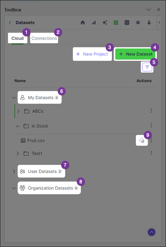 Shows all projects and project contents
Displays datasets previously uploaded to or downloaded from Anaconda's cloud storage
Create a new project to store and share datasets (sheets and tables)
Create a new dataset and assign it to a project
Apply filters to efficiently locate data in your catalog
A collection of all your cloud projects and their nested datasets
Projects to which you have access, owned by other individuals
Projects to which you have access, owned by organizations
Indicates the [connection status](#understanding-status-icons) of your dataset
Shows all projects and project contents
Displays datasets previously uploaded to or downloaded from Anaconda's cloud storage
Create a new project to store and share datasets (sheets and tables)
Create a new dataset and assign it to a project
Apply filters to efficiently locate data in your catalog
A collection of all your cloud projects and their nested datasets
Projects to which you have access, owned by other individuals
Projects to which you have access, owned by organizations
Indicates the [connection status](#understanding-status-icons) of your dataset
Creating a project
When you first access Datasets, you are prompted to create a new project. You can think of projects as folders for storing your datasets.
Create a project at any time using the following steps:
From the Cloud tab, click + New Project.
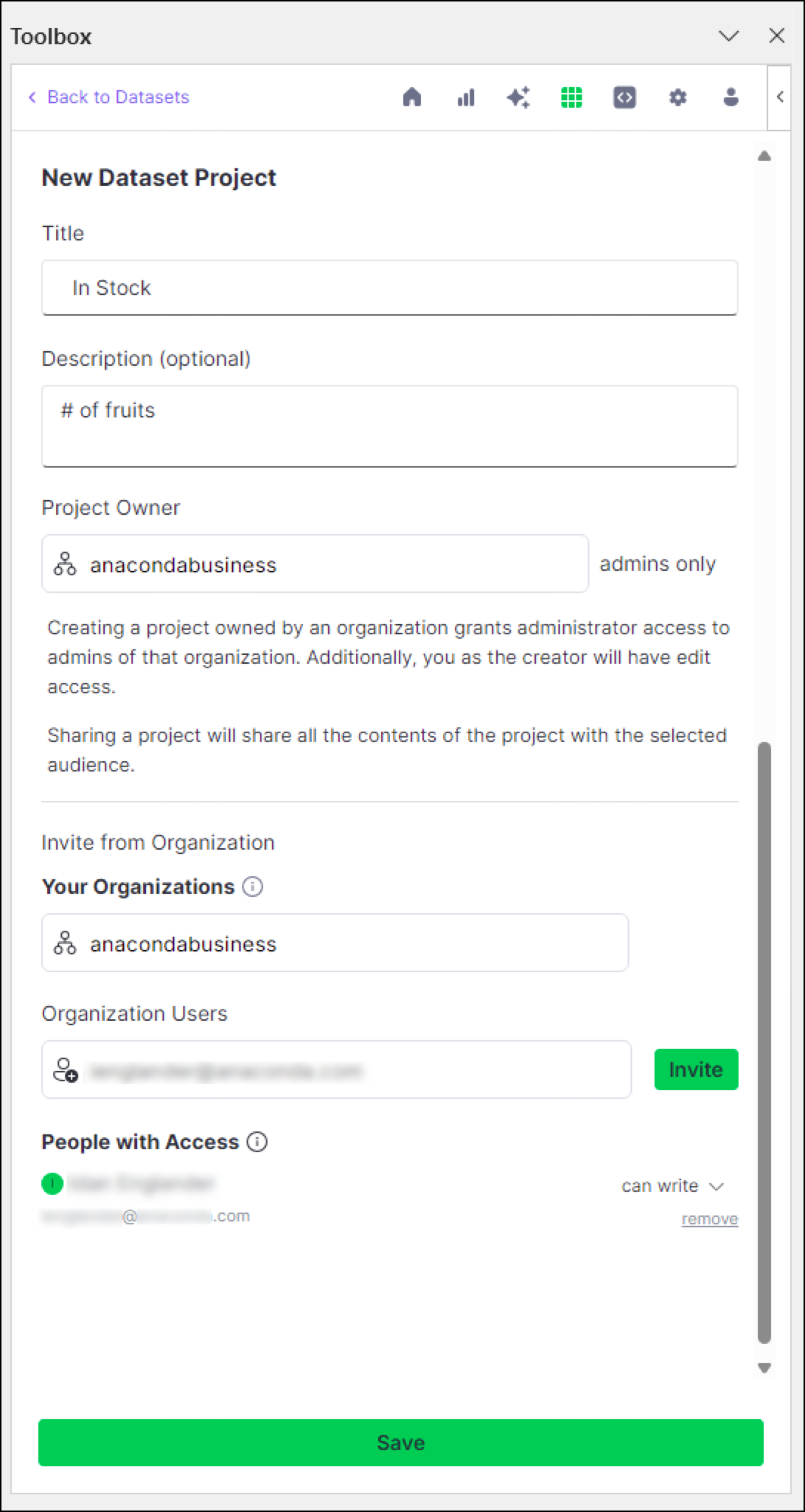
Enter a unique title for your project and an optional description.
Designate the project owner(s) for your project. By default, you are set as the only project owner.
Administrators and project owners are the only users allowed to edit projects. Anaconda.com organization administrators have full permissions for any projects owned by their organization.(Optional) Provide access to your project by inviting users from one of your organizations.
Click Save.
Sharing a project with other users
You can share a project to collaborate with others in your organization when creating a new project, or at any time using the following steps:
From the Cloud tab, click actions beside a project for which you have edit permissions, then click Edit.
Provide access to your project by inviting users from one of your organizations.
- Under Your Organizations, select an organization.
- Under Organization Users, select a user to share your project with.
- Choose whether the user should have read or write access to your project.
Click Save.
Permissions
Access to projects and the actions you can perform in them are determined by your permission level for the project. By default, you as the owner of your project have admin permissions; for projects owned by an organization, the admins of that organization have admin permissions for that project.
| Permission level | Actions |
|---|---|
| Read | View, download |
| Edit | View, download, upload |
| Admin | View, download, upload, share, delete |
Uploading data
Protect your local datasets and increase their accessibility by saving them in cloud storage. If you experience hardware failure, or need to work on a different device, your projects will be right where you left them!
Upload sheets and tables to your projects using the following steps:
From the Cloud tab, click + New Dataset.
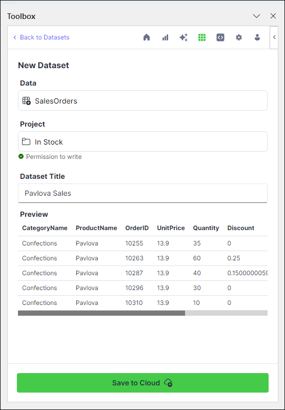
Under Data, choose a range of data manually, a specific table, or an entire sheet.
Under Project, select a project to house your dataset.
Under Dataset Title, provide a title for your dataset.
Complete the upload by clicking Save to Cloud.
You can now see the established connection between your dataset and Anaconda's cloud storage on the Connections tab.
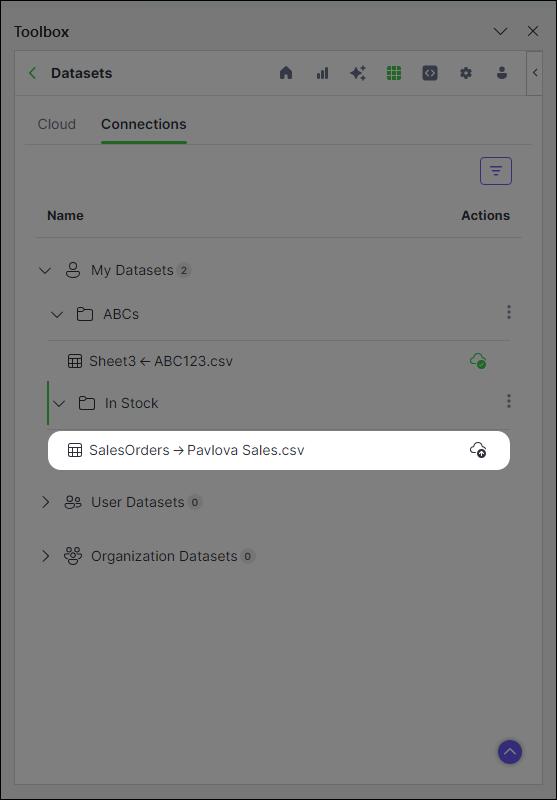
When you make changes to the dataset, re-upload it to update the dataset stored in the cloud.
Downloading data
If another user shares a project with you, or if you've uploaded a dataset in another workbook or Anaconda Notebook, download appears beside that dataset. Datasets can be downloaded as either an Excel range reference or as an Anaconda Code object.
To download a dataset as an Excel range reference:1. Click **download** beside the dataset you want to download.
2. Under **Workbook Placement**, select the sheet where you want to insert the data.
3. Complete the download by clicking **Download to Workbook**.
The data is now available in the selected sheet.
1. Click **download** beside the dataset you want to download.
2. Select **Import as Anaconda Code object**.

   <Note>
     If you're unable to select **Import as Anaconda Code object**, go to <Icon icon="gear" iconType="solid" /> **Settings** and, under **Generate Toolbox code as:**, select **Anaconda Code (=ANACONDA.CODE).**

     <Frame>
       <img src="https://mintcdn.com/anaconda-29683c67/opbTXGcYjx4zM8zO/images/generate_as_anaconda_code.png?fit=max&auto=format&n=opbTXGcYjx4zM8zO&q=85&s=5c7405100697762c86d0b68a43445670" alt="" data-og-width="1438" width="1438" data-og-height="684" height="684" data-path="images/generate_as_anaconda_code.png" data-optimize="true" data-opv="3" srcset="https://mintcdn.com/anaconda-29683c67/opbTXGcYjx4zM8zO/images/generate_as_anaconda_code.png?w=280&fit=max&auto=format&n=opbTXGcYjx4zM8zO&q=85&s=3435fd914dece65013aee11ea8bead7e 280w, https://mintcdn.com/anaconda-29683c67/opbTXGcYjx4zM8zO/images/generate_as_anaconda_code.png?w=560&fit=max&auto=format&n=opbTXGcYjx4zM8zO&q=85&s=c75b5c246de94c89e0f8f05730bfe95f 560w, https://mintcdn.com/anaconda-29683c67/opbTXGcYjx4zM8zO/images/generate_as_anaconda_code.png?w=840&fit=max&auto=format&n=opbTXGcYjx4zM8zO&q=85&s=a14e0dfd1991c96bb9832736252357f1 840w, https://mintcdn.com/anaconda-29683c67/opbTXGcYjx4zM8zO/images/generate_as_anaconda_code.png?w=1100&fit=max&auto=format&n=opbTXGcYjx4zM8zO&q=85&s=eda1e8da60a7636701e5d158f45dfa89 1100w, https://mintcdn.com/anaconda-29683c67/opbTXGcYjx4zM8zO/images/generate_as_anaconda_code.png?w=1650&fit=max&auto=format&n=opbTXGcYjx4zM8zO&q=85&s=14044f7db9686c41970447f94e835d76 1650w, https://mintcdn.com/anaconda-29683c67/opbTXGcYjx4zM8zO/images/generate_as_anaconda_code.png?w=2500&fit=max&auto=format&n=opbTXGcYjx4zM8zO&q=85&s=07c2360021872871f4b862a99a98ec59 2500w" />
     </Frame>
   </Note>
3. Click **Click to select**.
4. Select an empty cell.
5. Click **OK** in the Select Data dialog.
6. Click **Download to Workbook**.

The selected cell will display <Icon icon="cloud" iconType="regular" /> **PyScript Data**. Click <Icon icon="cloud" iconType="regular" /> to see details about the object.
Understanding status icons
Status icons appear by each dataset. Click the icons to perform the following functions:
| Icon | Name | Function |
|---|---|---|
| Upload | Click to upload a dataset in your workbook to Anaconda's cloud storage. | |
| Re-upload | Click to re-upload the dataset in your workbook to Anaconda's cloud storage. | |
| Download | Click to download a dataset from Anaconda's cloud storage to your workbook. | |
| Re-download | The dataset on Anaconda's cloud storage has been updated. Click to update the dataset in your Excel workbook with these changes. | |
| Synced | The dataset in your Excel workbook is up-to-date with the dataset in Anaconda's cloud storage. | |
| Conflict | The dataset on Anaconda's cloud storage has been updated and now conflicts with the dataset in your Excel Workbook. Click to resolve the conflict. |
Code Snippets
Code Snippets enable you to securely upload reusable blocks of code to Anaconda's cloud storage. You can then provide access to other users, as well as import your code snippets to separate workbooks to repeat your efforts from any machine, anytime.
Understanding connections
Let's take a look at the different elements within Code Snippets.
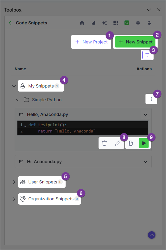 Create a new project to store and share snippets
Create and store a new snippet in Anaconda's cloud storage
Apply filters to efficiently locate snippets in your catalog
A collection of all your cloud projects and their nested snippets
Projects to which you have access, owned by other individuals
Projects to which you have access, owned by organizations
Edit, delete, and [share projects](#sharing-a-snippet)
Edit and delete snippets
Multiple methods for [adding and running snippets in a workbook](#adding-snippets-to-a-workbook)
Create a new project to store and share snippets
Create and store a new snippet in Anaconda's cloud storage
Apply filters to efficiently locate snippets in your catalog
A collection of all your cloud projects and their nested snippets
Projects to which you have access, owned by other individuals
Projects to which you have access, owned by organizations
Edit, delete, and [share projects](#sharing-a-snippet)
Edit and delete snippets
Multiple methods for [adding and running snippets in a workbook](#adding-snippets-to-a-workbook)
Create a project
When you first access Code Snippets, you are prompted to create a new project. You can think of projects as folders for storing your snippets.
You must create a project before uploading your first snippet. Create a project at any time using the following steps:
Click + New Project.
Enter a unique title for your project and an optional description.
Designate the project owner(s) for your project. By default, you are set as the only project owner.
Administrators and project owners are the only users allowed to edit projects. Anaconda.com organization administrators have full permissions for any projects owned by their organization.(Optional) Provide access to your project by inviting users from one of your organizations.
Click Save.
Sharing a snippet
You can share a snippet with others in your organization by sharing the project containing that snippet. This can be done as you're creating a new project or at any time using the following steps:
Click actions beside a project for which you have edit permissions, then click Edit.
Provide access to your project by inviting users from one of your organizations.
- Under Your Organizations, select an organization.
- Under Organization Users, select a user to share your project with.
- Choose whether the user should have read or write access to your project.
Click Save.
Uploading a snippet
With a project in Anaconda's cloud storage, you can now create a snippet and upload it to that project. This can be done from Code Snippets or, if you want to save code generated while creating visualizations of your data, you can upload a snippet from Visualize with Python.
1. Click **+ New Snippet**. 2. Under **Project**, select an existing project to house your snippet. 3. Under **Snippet Title**, provide a title for your snippet. 4. Select a language, then enter your code in the code editor. Alternatively, click **+ Add From Grid** to add existing code from your workbook. 5. Click **Save to Cloud**.Your snippet appears in its assigned project folder.
1. From the Toolbox home screen, open **Visualize with Python**.

2. Click **New Chart**, then select a chart type.

3. Select the source range and adjust the chart settings from the **Setup** tab, customize the chart from the **Design** tab, and then open the **Code** tab.

4. Click <Icon icon="rectangle-code" iconType="regular" /> **Save as code snippet** to open the code in Code Snippets.

   <Frame>
     <img src="https://mintcdn.com/anaconda-29683c67/u4MsRLDCM8Pedgc_/images/snippets_visualize.png?fit=max&auto=format&n=u4MsRLDCM8Pedgc_&q=85&s=c43c7d207802a7b65227362aa973e0fd" alt="" data-og-width="535" width="535" data-og-height="800" height="800" data-path="images/snippets_visualize.png" data-optimize="true" data-opv="3" srcset="https://mintcdn.com/anaconda-29683c67/u4MsRLDCM8Pedgc_/images/snippets_visualize.png?w=280&fit=max&auto=format&n=u4MsRLDCM8Pedgc_&q=85&s=e649649a63fff8080c8f9637650b9887 280w, https://mintcdn.com/anaconda-29683c67/u4MsRLDCM8Pedgc_/images/snippets_visualize.png?w=560&fit=max&auto=format&n=u4MsRLDCM8Pedgc_&q=85&s=de305391a3feb6f6d975c15d1a57a4a8 560w, https://mintcdn.com/anaconda-29683c67/u4MsRLDCM8Pedgc_/images/snippets_visualize.png?w=840&fit=max&auto=format&n=u4MsRLDCM8Pedgc_&q=85&s=2f7feb3a15309125e8ac13751472e25a 840w, https://mintcdn.com/anaconda-29683c67/u4MsRLDCM8Pedgc_/images/snippets_visualize.png?w=1100&fit=max&auto=format&n=u4MsRLDCM8Pedgc_&q=85&s=8cfd56f3b927491983be90776f411be8 1100w, https://mintcdn.com/anaconda-29683c67/u4MsRLDCM8Pedgc_/images/snippets_visualize.png?w=1650&fit=max&auto=format&n=u4MsRLDCM8Pedgc_&q=85&s=fd4b5a0b79a5e4b9392605e8fc589f63 1650w, https://mintcdn.com/anaconda-29683c67/u4MsRLDCM8Pedgc_/images/snippets_visualize.png?w=2500&fit=max&auto=format&n=u4MsRLDCM8Pedgc_&q=85&s=765843202c5339529fe319d2e7b9c1f6 2500w" />
   </Frame>

5. Select a project to upload the snippet to, then provide a title.

6. If needed, edit the code to suit multiple use cases by converting labels to variables, parameterizing functions, and so on.

7. Click **Save to Cloud**.

Your snippet appears in its assigned project folder.
Adding snippets to a workbook
When you're ready to make use of your saved snippets, import them to a workbook using the following steps:
Expand the dropdown beside your snippet. A preview of your snippet appears.
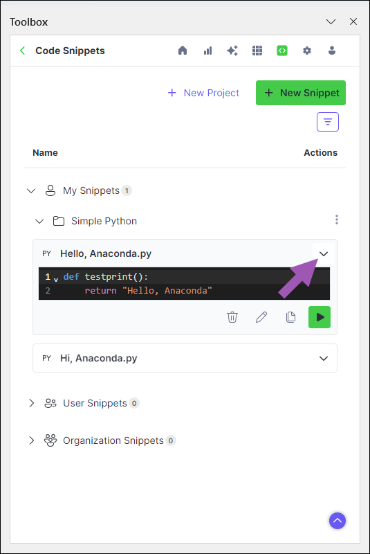
You can now import your snippet in one of two ways:
Editing a snippet
Changes made to a saved snippet in a workbook will not automatically update that snippet in Anaconda's cloud storage. Instead, you must make changes to the snippet directly within the Anaconda Toolbox extension.
Expand the dropdown beside your snippet. A preview of your snippet appears.
Click Edit.
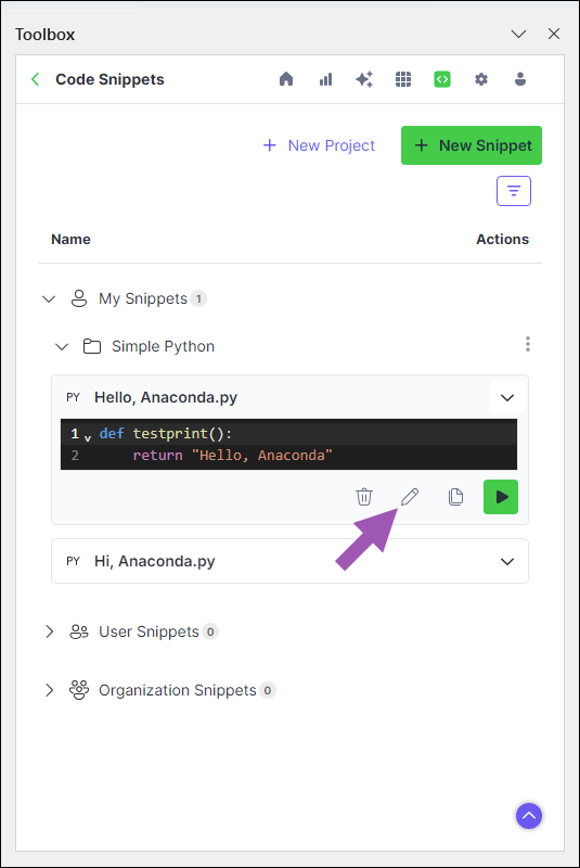
Adjust your snippet, then click Save to Cloud.
Changing the title of your snippet will create a new snippet, rather than updating the existing one.
Code Snippets
Code Snippets enable you to securely upload reusable blocks of code to Anaconda's cloud storage. You can then provide access to other users, as well as import your code snippets to separate workbooks to repeat your efforts from any machine, anytime.
Understanding connections
Let's take a look at the different elements within Code Snippets.
Create a new project to store and share snippets
Create and store a new snippet in Anaconda's cloud storage
Apply filters to efficiently locate snippets in your catalog
A collection of all your cloud projects and their nested snippets
Projects to which you have access, owned by other individuals
Projects to which you have access, owned by organizations
Edit, delete, and [share projects](#sharing-a-snippet)
Edit and delete snippets
Multiple methods for [adding and running snippets in a workbook](#adding-snippets-to-a-workbook)
Create a project
When you first access Code Snippets, you are prompted to create a new project. You can think of projects as folders for storing your snippets.
You must create a project before uploading your first snippet. Create a project at any time using the following steps:
Click + New Project.
Enter a unique title for your project and an optional description.
Designate the project owner(s) for your project. By default, you are set as the only project owner.
Administrators and project owners are the only users allowed to edit projects. Anaconda.com organization administrators have full permissions for any projects owned by their organization.(Optional) Provide access to your project by inviting users from one of your organizations.
Click Save.
Sharing a snippet
You can share a snippet with others in your organization by sharing the project containing that snippet. This can be done as you're creating a new project or at any time using the following steps:
Click actions beside a project for which you have edit permissions, then click Edit.
Provide access to your project by inviting users from one of your organizations.
- Under Your Organizations, select an organization.
- Under Organization Users, select a user to share your project with.
- Choose whether the user should have read or write access to your project.
Click Save.
Uploading a snippet
With a project in Anaconda's cloud storage, you can now create a snippet and upload it to that project. This can be done from Code Snippets or, if you want to save code generated while creating visualizations of your data, you can upload a snippet from Visualize with Python.
1. Click **+ New Snippet**. 2. Under **Project**, select an existing project to house your snippet. 3. Under **Snippet Title**, provide a title for your snippet. 4. Select a language, then enter your code in the code editor. Alternatively, click **+ Add From Grid** to add existing code from your workbook. 5. Click **Save to Cloud**.Your snippet appears in its assigned project folder.
1. From the Toolbox home screen, open **Visualize with Python**.

2. Click **New Chart**, then select a chart type.

3. Select the source range and adjust the chart settings from the **Setup** tab, customize the chart from the **Design** tab, and then open the **Code** tab.

4. Click <Icon icon="rectangle-code" iconType="regular" /> **Save as code snippet** to open the code in Code Snippets.

   <Frame>
     <img src="https://mintcdn.com/anaconda-29683c67/u4MsRLDCM8Pedgc_/images/snippets_visualize.png?fit=max&auto=format&n=u4MsRLDCM8Pedgc_&q=85&s=c43c7d207802a7b65227362aa973e0fd" alt="" data-og-width="535" width="535" data-og-height="800" height="800" data-path="images/snippets_visualize.png" data-optimize="true" data-opv="3" srcset="https://mintcdn.com/anaconda-29683c67/u4MsRLDCM8Pedgc_/images/snippets_visualize.png?w=280&fit=max&auto=format&n=u4MsRLDCM8Pedgc_&q=85&s=e649649a63fff8080c8f9637650b9887 280w, https://mintcdn.com/anaconda-29683c67/u4MsRLDCM8Pedgc_/images/snippets_visualize.png?w=560&fit=max&auto=format&n=u4MsRLDCM8Pedgc_&q=85&s=de305391a3feb6f6d975c15d1a57a4a8 560w, https://mintcdn.com/anaconda-29683c67/u4MsRLDCM8Pedgc_/images/snippets_visualize.png?w=840&fit=max&auto=format&n=u4MsRLDCM8Pedgc_&q=85&s=2f7feb3a15309125e8ac13751472e25a 840w, https://mintcdn.com/anaconda-29683c67/u4MsRLDCM8Pedgc_/images/snippets_visualize.png?w=1100&fit=max&auto=format&n=u4MsRLDCM8Pedgc_&q=85&s=8cfd56f3b927491983be90776f411be8 1100w, https://mintcdn.com/anaconda-29683c67/u4MsRLDCM8Pedgc_/images/snippets_visualize.png?w=1650&fit=max&auto=format&n=u4MsRLDCM8Pedgc_&q=85&s=fd4b5a0b79a5e4b9392605e8fc589f63 1650w, https://mintcdn.com/anaconda-29683c67/u4MsRLDCM8Pedgc_/images/snippets_visualize.png?w=2500&fit=max&auto=format&n=u4MsRLDCM8Pedgc_&q=85&s=765843202c5339529fe319d2e7b9c1f6 2500w" />
   </Frame>

5. Select a project to upload the snippet to, then provide a title.

6. If needed, edit the code to suit multiple use cases by converting labels to variables, parameterizing functions, and so on.

7. Click **Save to Cloud**.

Your snippet appears in its assigned project folder.
Adding snippets to a workbook
When you're ready to make use of your saved snippets, import them to a workbook using the following steps:
Expand the dropdown beside your snippet. A preview of your snippet appears.
You can now import your snippet in one of two ways:
Editing a snippet
Changes made to a saved snippet in a workbook will not automatically update that snippet in Anaconda's cloud storage. Instead, you must make changes to the snippet directly within the Anaconda Toolbox extension.
Expand the dropdown beside your snippet. A preview of your snippet appears.
Click Edit.
Adjust your snippet, then click Save to Cloud.
Changing the title of your snippet will create a new snippet, rather than updating the existing one.
Data Science & AI Workbench
Workbench is an enterprise-ready, secure and scalable data science platform that empowers teams to govern data science assets, collaborate and deploy their data science projects.
With Workbench, you can do the following:
- Develop: ML/AI pipelines in a central development environment that scales from laptops to thousands of nodes
- Govern: Complete reproducibility from laptop to cluster with the ability to configure access control
- Automate: Model training and deployment on scalable, container-based infrastructure
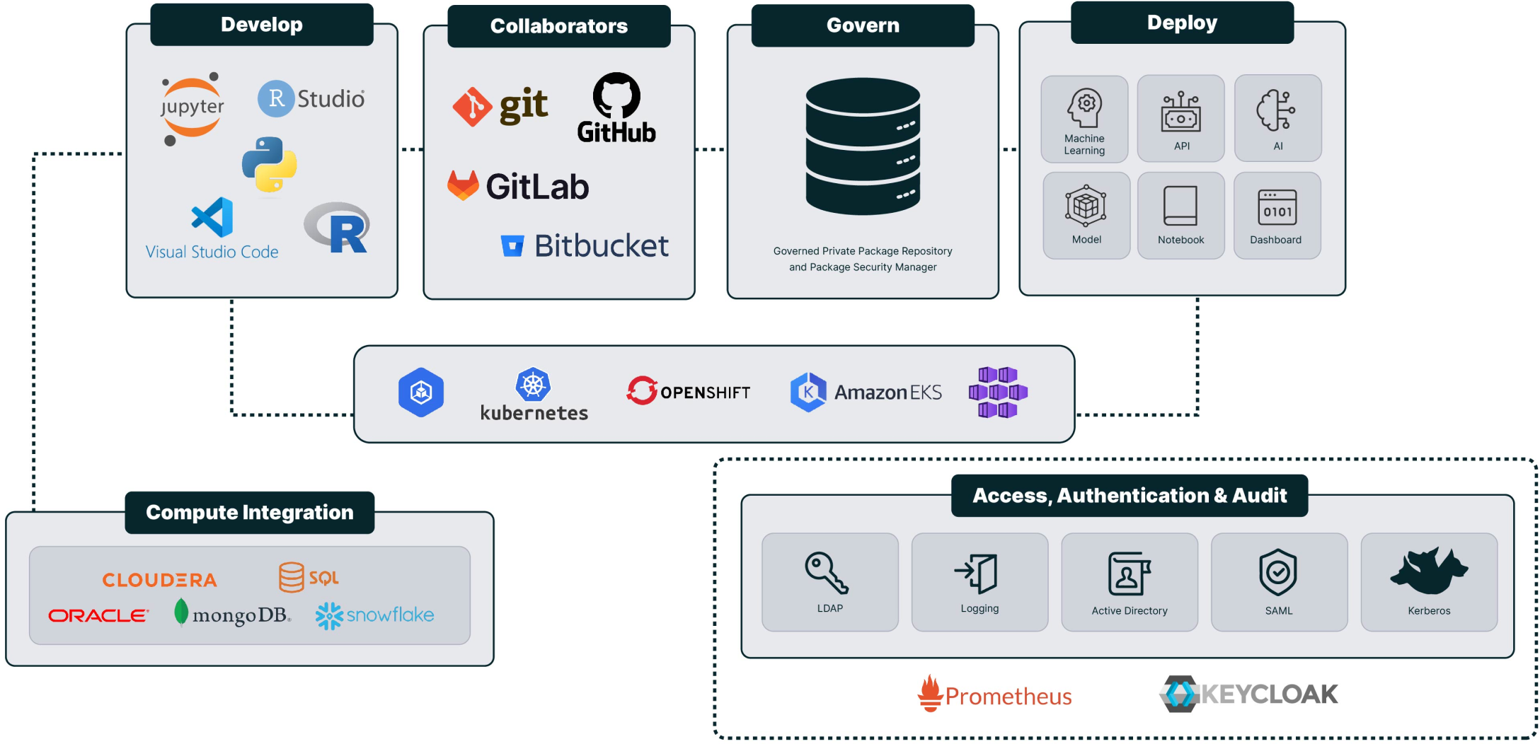
Using Workbench
Using Workbench
Project configurations
In Data Science & AI Workbench, projects are structured around a core configuration file called anaconda-project.yml. This file is crucial for orchestrating a project’s components for deployment and ensuring operational consistency over time. There are several parameters that must be included within each project’s anaconda-project.yml file to ensure that it operates as intended:
- Packages - You must specify all conda or pip packages the project requires to function in its
anaconda-project.ymlfile. By default, Workbench is configured to use packages from its internal repository to create project environments. However, it is possible to use packages from external repositories. - Environment - You must define at least one named environment to accurately manage the project’s packages and their dependencies, ensuring stability across different settings. Projects use template environments when they are initially created, which can be updated or replaced. For more information about template environments, see Configuring persistent environments and sample projects.
- Commands - You must define at least one command to properly deploy and run jobs for your project in its intended environment.
- Environmental variables - If necessary, set up the required environment variables needed to control how your project interacts with external resources and services.
Instead, Anaconda recommends using anaconda-project commands from a terminal within your project to update its configurations when possible. For more information about anaconda-project, see the official documentation here.
All anaconda-project commands must be run from the lab_launch environment! Enter the lab_launch environment by running the following command in a project terminal:
conda activate lab_launch
Once you are finished configuring your project, Anaconda recommends that you add a lock file to your project to ensure its reproducibility across different environments at scale.
Configuring project environments
The conda environments in standard project templates are pre-solved to reduce initialization time when additional packages are added. However, you might want to create an environment specifically for your project.
To create a new environment with specific packages and add it to your project:
Create a new project.
Start a session.
Open a terminal within your session editor.
Create an environment and include the packages you need for it by running the following command:
 # Replace <ENV_NAME> with the name of the environment you are creating to add to your project's configuration
 # Replace <PACKAGE_NAME> with the name of the packages you want to add to your project's configuration
 anaconda-project add-env-spec --name <ENV_NAME> <PACKAGE_NAME> <PACKAGE_NAME>
Remove the template environment that you used to create your project by running the following command:
# Replace <TEMPLATE_ENV> with the name of the template environment you used to initially create the project anaconda-project remove-env-spec --name <TEMPLATE_ENV>Stop and re-start the project.
   ```sh  theme={null}
   cd /opt/continuum/
   ls
   ```

   If the environment is being initialized, you will see a file named `preparing`. Once initialization is complete, you will see a file named `prepare.log`. To troubleshoot environment initialization, view the log from the terminal by running the following command:

   ```sh  theme={null}
   cat /opt/continuum/prepare.log
   ```
Configuring project packages
Adding a package to a project’s configuration file persists for future project sessions and deployments. This is different than using conda install to add a package using the conda environment during a session, which impacts the project during the current session only.
Adding conda packages
To add a conda package to your project’s anaconda-project.yml file:
Open your project.
If necessary, start a session.
Open a terminal within your session editor.
Verify that you are in the
lab_launchenvironment.Run the following command:
```sh theme={null} # Replace with the name of the packages you want to add to your project's configuration anaconda-project add-packages ``` ```sh theme={null} # Replace with the name of the channel that contains the packages you want to add # Replace with the name of the packages you want to add to your project's configuration anaconda-project add-packages --channel ``` To use packages from an external repository, you will need to specify the full channel URL in the command:```sh theme={null} # Replace <CHANNEL_URL> with the address of the channel that contains the packages you want to add # Replace <PACKAGE_NAME> with the name of the packages you want to add to your project's configuration anaconda-project add-packages <PACKAGE_NAME> --channel <CHANNEL_URL> ```The command may take a moment to run as it solves the environment to collect dependencies and download packages. Once complete, the added packages appear in the project’s
anaconda-project.ymlfile. If the file is open when you run the command, close and reopen it to view your changes.Stop and re-start the project session.
Adding pip packages
If your project requires you to pip install a package, you can use anaconda-project to add it to your project’s configuration.
To add a pip package to your project’s anaconda-project.yml file:
Open your project.
If necessary, start a session.
Open a terminal within your session editor.
Verify that you are in the
lab_launchenvironment.Run the following command:
# Replace <PACKAGE_NAME> with the name of the packages you want to add to your project's configuration anaconda-project add-packages --pip <PACKAGE_NAME> <PACKAGE_NAME>Stop and re-start the project session.
Removing packages
To remove a package from your project’s anaconda-project.yml file:
Open your project.
If necessary, start a session.
Open a terminal within your session editor.
Verify that you are in the
lab_launchenvironment.Run the following command:
# Replace <PACKAGE_NAME> with the name of the packages you want to remove from your project's configuration anaconda-project remove-packages <PACKAGE_NAME> <PACKAGE_NAME>Stop and re-start the project session.
Configuring project environment variables
Environment variables are key parameters that manage dynamic settings like API keys, database URLs, and memory limits without modifying the codebase. These variables are essential for deploying projects consistently.
To add environment variables with a default value to your project’s anaconda-project.yml file:
Open your project.
If necessary, start a session.
Open a terminal within your session editor.
Verify that you are in the
lab_launchenvironment.Run the following command:
# Replace <VALUE> with the content of your environment variable # Replace <VARIABLE> with the variable name anaconda-project add-variable --default=<VALUE> <VARIABLE>Stop and re-start the project session.
For more information and advanced command arguments, see Working with environment variables in the official anaconda-project documentation.
Configuring project commands
To deploy a project in Workbench, it must contain at least one appropriate deployment command defined in its anaconda-project.yml file. These commands specify how the project’s components, such as notebooks, scripts, or generic web frameworks, should be executed when the project is deployed.
To add a command to your project’s anaconda-project.yml file:
Open your project.
If necessary, start a session.
Open a terminal within your session editor.
Verify that you are in the
lab_launchenvironment.Run the following command:
# Replace <CMD_NAME> with a name for your deployment command # Replace <COMMAND> with the project filename that should be executed anaconda-project add-command <CMD_NAME> <COMMAND>Stop and re-start the project session.
For more information and advanced command arguments, see Working with commands in the official anaconda-project documentation.
For a Notebook:
commands:
default:
   notebook: <FILE_NAME>.ipynb
For a Panel dashboard:
commands:
default:
   unix: panel serve <SCRIPT_OR_NOTEBOOK_FILE>
   supports_http_options: True
For a generic script or web framework, including Python or R:
commands:
default:
   unix: bash <YOUR-SCRIPT>.sh
   supports_http_options: true
commands:
default:
   unix: python <YOUR-SCRIPT>.py
   supports_http_options: true
commands:
default:
   unix: Rscript <YOUR-SCRIPT>.R
   supports_http_options: true
Validating project deployment commands
To validate the anaconda-project.yml and verify your project will deploy successfully:
Open your project.
If necessary, start a session.
Open a terminal within your session editor.
Verify that you are in the
lab_launchenvironment.Prepare the environment and test the deployment command by running the following commands:
# Replace <ENV_NAME> with the name of the project's environment
# Replace <COMMAND> with the deployment command that you want to test
anaconda-project prepare --env-spec <ENV_NAME>
anaconda-project run <COMMAND>
Any errors preventing a successful deployment are displayed in the terminal.
Testing project deployments
Once deployment commands are added to your project, you can test the deployment using the test_deployment command. This sets up a mini web application, allowing you to preview your deployment locally using a port within your session.
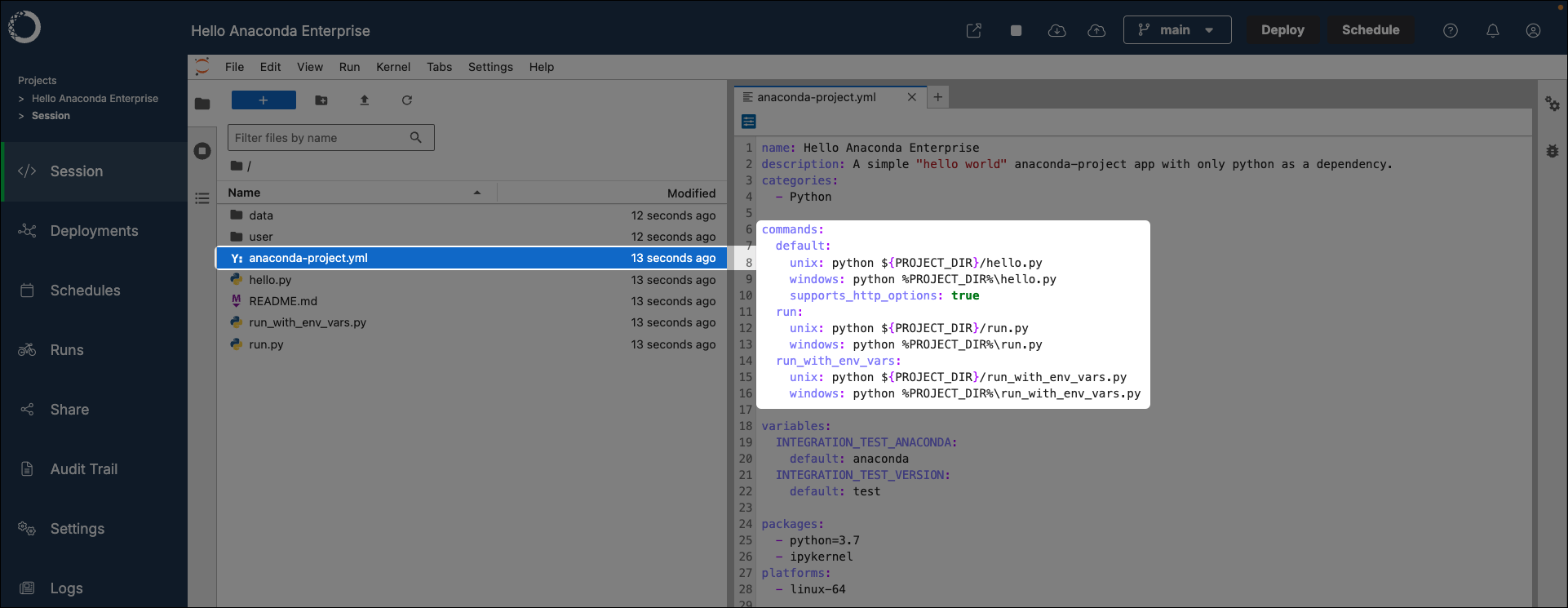
To test a project deployment:
Open your project.
If necessary, start a session.
Open a terminal within your session editor.
Verify that you are in the
lab_launchenvironment.Test a deployment command you’ve added to your project by running the following command:
# Replace <COMMAND> with an available deployment command test_deployment <COMMAND>Navigate to the web address returned by the command to verify your project deployed successfully.
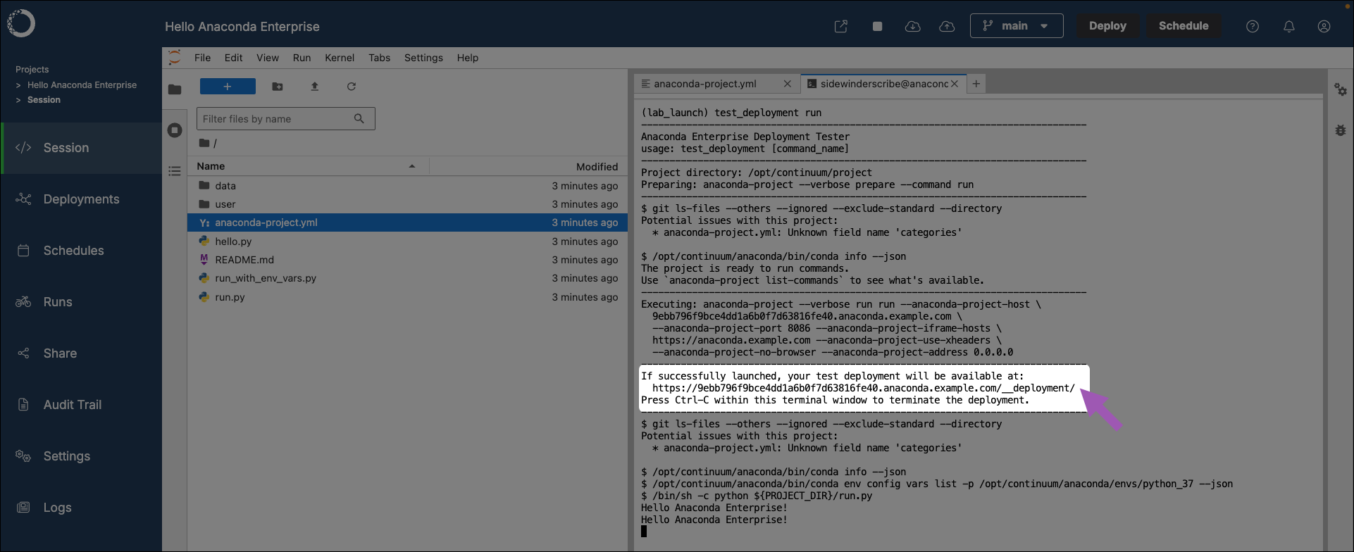
Locking project configurations
Project locking is a crucial step in ensuring your project is reproducible across multiple deployments at scale. It is best practice to lock your project once you have finalized configurations for your project, or if you are preparing to transition to a production or public deployment. For more information, see Project reproducibility in Workbench.
To lock your anaconda-project.yml file configurations to a fixed state:
Open your project.
If necessary, start a session.
Open a terminal within your session editor.
Verify that you are in the
lab_launchenvironment.Lock your project configurations by running the following command:
anaconda-project lock
This instructs conda to solve the project’s environment, lock all packages and their dependencies to their current versions, and generates an anaconda-project-lock.yml file for your project.
Project logs
Because Data Science & AI Workbench is built on top of a Kubernetes cluster, each project session is created as a pod. Each project session pod has an editor, sync, and proxy container, and logs for each container are accessible to aid you in troubleshooting issues you may encounter with your project. These logs can provide insights to the operational health of your project, possible configuration errors, and potential security issues.
Viewing project logs
To view a project session’s logs:
- Log in to Workbench.
- Open a project.
- If necessary, start a session in the project.
- Select Logs from the left-hand navigation.
- Open a container dropdown to view the logs for that container.
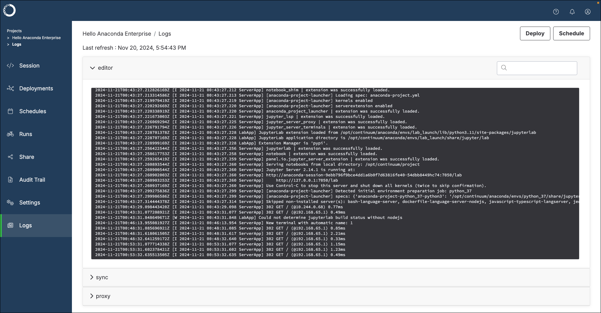 Use **Search** to help you efficiently locate information in the container logs.
Editor container logs
The editor container is where the integrated development environment (IDE) set by the project configurations runs. Logs from this container can provide insights into the following:
- User actions performed within the editor, such as file edits, saves, and execution of code cells
- Errors or warnings related to the editor software, as opposed to Workbench software
- Problems that are caused by editor plug-ins or extensions
Sync container logs
The sync container is responsible for synchronizing project files and code between persistent storage and the editor. Logs from this container can provide insights into the following:
- Successes or failures when syncing files between the local user repository and the projects remote repository
- Issues encountered during file creation or deletion, or file modification attempts
- Problems accessing external resources the project relies on
Proxy container logs
The proxy container handles network traffic to and from the project’s environment, and facilitates access to web interfaces and APIs. Logs from this container can provide insights into the following:
- Incoming and outgoing network requests, which is useful for identifying unauthorized access attempts
- Errors related to network connectivity, DNS issues, or failed attempts to connect to external services
- Information on request handling times and bottlenecks in network communication
Visualizations and dashboards
Data Science & AI Workbench makes it easy for you to create and share interactive data visualizations, live notebooks or machine learning models built using popular libraries such as Bokeh and HoloViews.
To get you started quickly, Workbench provides sample projects of Bokeh applications for clustering and cross filtering data. There are also several examples of Workbench projects that use HoloViz here.
Create an interactive plot
From the Projects view, create a new project using the minimal Python templates:
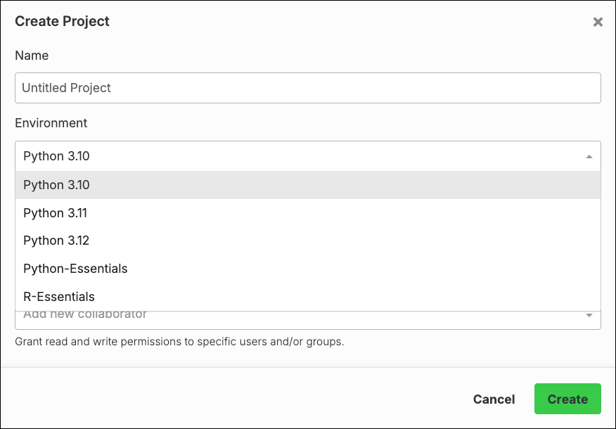
Open a session for your newly created project.
Open a terminal.
Run the following command to install
hvplotandpanel:anaconda-project add-packages hvplot panelCreate a new Notebook and rename it to
tips.ipynb.Add the following code to
tips.ipynb:import pandas as pd import hvplot.pandas import panel panel.extension() df = pd.read_csv('http://bit.ly/tips-csv') p = df.hvplot.scatter(x='total_bill', y='tip', hover_cols=['sex','day','size']) pn.panel(p).servable()Open the project’s
anaconda-project.ymlfile, and add the following deployment command:commands: scatter-plot: unix: panel serve tips.ipynb supports_http_options: True
export const AnacondaIcon = () => { return ; };
In Anaconda Notebooks, a runtime is what powers your code execution. You can think of a runtime as a conda environment connected to a language-specific kernel. Anaconda Notebooks provides several pre-configured runtimes that include the ipykernel package and all the packages from the latest Anaconda Distribution release, giving you immediate access to a comprehensive data science toolkit.
Environments, kernels, and runtimes
What is an environment?
An environment is a folder or directory that contains a specific collection of conda packages and their dependencies.
Working in separate environments allows you to maintain and run packages without interference from other collections of packages. For example, you may require separate conda environments to maintain distinct versions of Python based on distinct package dependencies.
What is a kernel?
A kernel is a programming-language-specific process that interprets your code, runs it, and gives you the results. In Jupyter Notebooks, kernels allow users to run code in cells and receive immediate output. For example, ipykernel enables interactive computing in Python.
What is a runtime?
A runtime in Anaconda Notebooks is a conda environment that has been associated with a specific kernel, enabling it to execute code. For an environment to be usable in JupyterLab, it must contain a kernel package (such as ipykernel for Python). Without this kernel association, JupyterLab cannot recognize the environment as an available option for running notebooks.
The default runtimes provided in Anaconda Notebooks come with the ipykernel package already installed, making them immediately available for your Python notebooks.
To add a kernel package to a custom environment and create your own runtime, see creating custom runtimes.
Using default runtimes
Custom runtimes often use large amounts of your limited Anaconda Notebooks storage space. Because of this, Anaconda provides a number of read-only default runtimes that contain all the packages from the latest release of Anaconda Distribution.
The default runtime naming convention is typically anaconda-<YEAR>.<MONTH>-py<PYTHON_VERSION>, which maps to Anaconda Distribution releases:
| Environment Name | Status | Description |
|---|---|---|
| anaconda-2024.02-py10 | Live | Latest Anaconda Packages (stable & recommended) |
| anaconda-ai-2024.04-py10 | Live | Latest Anaconda Packages + AI Packages |
| anaconda-01-nvidia-a10 | Live | Latest Anaconda, AI, + NVIDIA Packages (see GPU Runtimes) |
To see a list of available runtimes, enter the following in a notebook cell then click Run:
!conda info --envs
To see a list of packages in your current runtime, enter the following in a notebook cell then click Run:
!conda list
Creating custom runtimes
If you need a specific set of packages that are not included in one of our default runtimes, you can create your own runtime to customize to your needs.
Custom runtimes are stored using your dedicated, persistent Anaconda Notebooks cloud storage. This ensures the custom runtime remains available after your current session ends. Custom runtimes use your personal storage space and can easily get quite large, so *only include the packages you need*.To create a new runtime:
Open a terminal from the Launcher, which you can access by selecting the blue plus in the top-left corner of the File Browser.
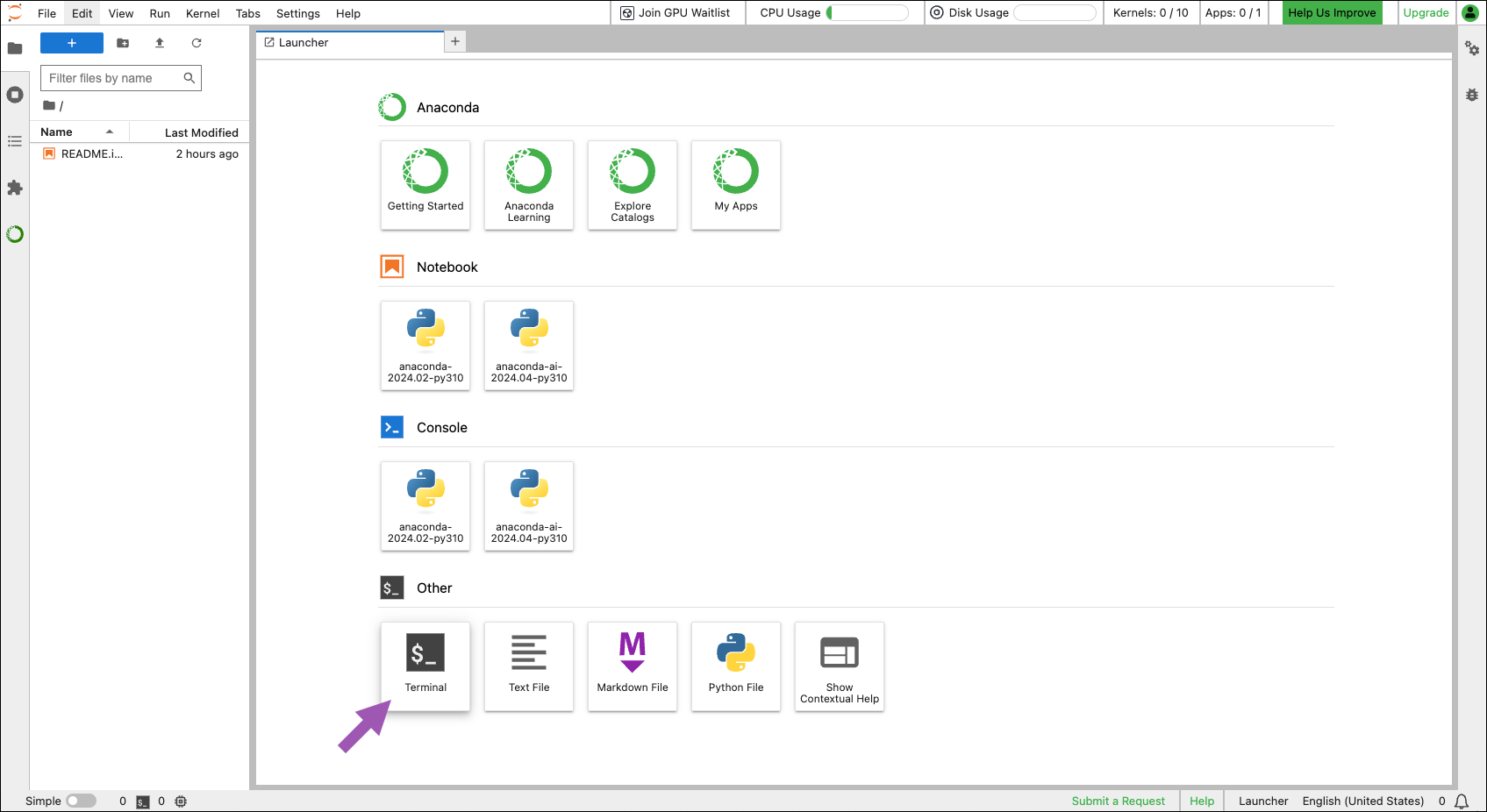
Create a new runtime by running the following command:
# Replace <ENV_NAME> with a new name for your environment/ runtime
# Replace <PACKAGE> with the name of a package you want to install in your environment
conda create --name <ENV_NAME> <PACKAGE> ipykernel
For more information about creating conda environments, see the official conda docs.
Creating a custom runtime from an environment.yml file
This feature is only available for the [local version of Toolbox](/tools/anaconda-notebooks/anaconda-toolbox/local-toolbox).If you have an existing environment.yml file, you can create a custom runtime by uploading it to an Anaconda Toolbox project and installing it directly from there.
Uploading an environment.yml file
Launch Anaconda Notebooks and select the left-side Anaconda Toolbox icon.
Select Manage Projects.
Select actions beside the project where you want to add your
environment.ymlfile, then select Upload.Select the
The dependencies list must include the `ipykernel` package.environment.ymlfile you want to create a custom runtime from. You can use any filename, but the file extension must be.yml.
The
environment.ymlfile must be in valid YAML format.
If your
environment.ymlfile includes aname:key, it will be removed during upload. You'll name your environment during installation.See the official conda docs for more information on creating an
environment.ymlfile.Select Upload to Project.
See Anaconda Projects for more details on creating projects and uploading files.
Installing the custom runtime
Navigate to the project where you uploaded the
environment.ymlfile.Select Install beside the
environment.ymlfilename.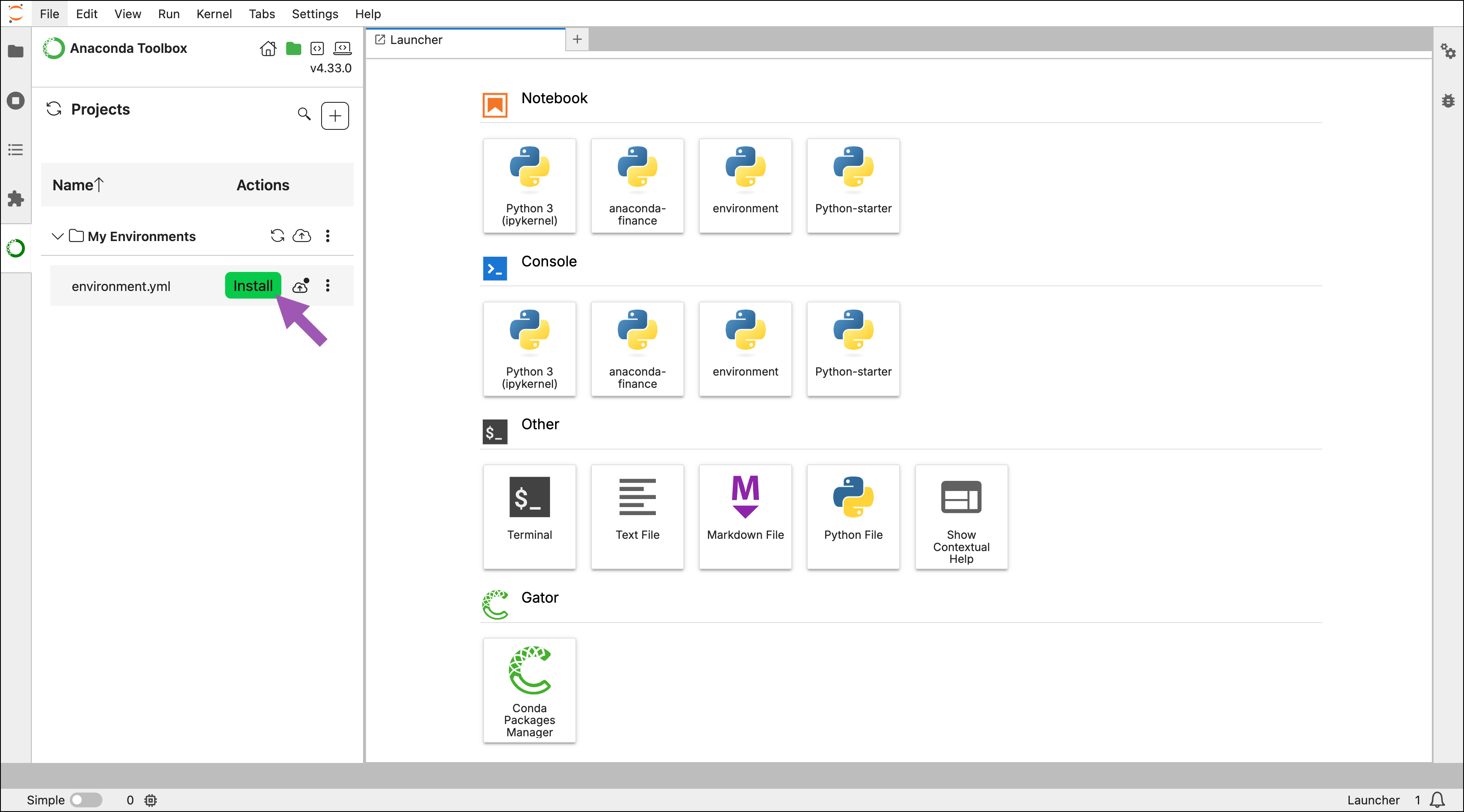
In the modal that appears, choose a unique name for your environment, then select Install.
Once installation is complete, an Edit environment button appears beside the filename.
Selecting Edit environment lets you edit your environment with the Gator environment manager.
Follow the steps in Activating a runtime to activate your custom runtime.
If installation fails, select Copy error logs beside the filename to troubleshoot. The most common issue is missing the required ipykernel package in your dependencies list.
Activating runtimes
There are a few locations from which you can activate a runtime:
1. Open a terminal from the Launcher.2. Run the following command:
```sh theme={null}
# Replace <ENV_NAME> with the name of your environment/ runtime
conda activate <ENV_NAME>
```
<Frame>
  <img src="https://mintcdn.com/anaconda-29683c67/q5KdI2mr6ZKMYRZp/images/notebook_launcher-env.png?fit=max&auto=format&n=q5KdI2mr6ZKMYRZp&q=85&s=9083cb734e9e83fe9dac0e40dda8ff6d" alt="" data-og-width="1730" width="1730" data-og-height="926" height="926" data-path="images/notebook_launcher-env.png" data-optimize="true" data-opv="3" srcset="https://mintcdn.com/anaconda-29683c67/q5KdI2mr6ZKMYRZp/images/notebook_launcher-env.png?w=280&fit=max&auto=format&n=q5KdI2mr6ZKMYRZp&q=85&s=545df58864877eb820556b8e8c6e2ddb 280w, https://mintcdn.com/anaconda-29683c67/q5KdI2mr6ZKMYRZp/images/notebook_launcher-env.png?w=560&fit=max&auto=format&n=q5KdI2mr6ZKMYRZp&q=85&s=b0cfa24e34cf7c425dc200117c9c24ee 560w, https://mintcdn.com/anaconda-29683c67/q5KdI2mr6ZKMYRZp/images/notebook_launcher-env.png?w=840&fit=max&auto=format&n=q5KdI2mr6ZKMYRZp&q=85&s=d64a1d90abde33f72f3391fbb9d102e7 840w, https://mintcdn.com/anaconda-29683c67/q5KdI2mr6ZKMYRZp/images/notebook_launcher-env.png?w=1100&fit=max&auto=format&n=q5KdI2mr6ZKMYRZp&q=85&s=8da71b19dc7a4cd2c6178515d5591af6 1100w, https://mintcdn.com/anaconda-29683c67/q5KdI2mr6ZKMYRZp/images/notebook_launcher-env.png?w=1650&fit=max&auto=format&n=q5KdI2mr6ZKMYRZp&q=85&s=13d87b9adf0f53bc35b3a8a864befaef 1650w, https://mintcdn.com/anaconda-29683c67/q5KdI2mr6ZKMYRZp/images/notebook_launcher-env.png?w=2500&fit=max&auto=format&n=q5KdI2mr6ZKMYRZp&q=85&s=9031b1773d5f1cce6df558349fca5579 2500w" />
</Frame>
<Frame>
  <img src="https://mintcdn.com/anaconda-29683c67/q5KdI2mr6ZKMYRZp/images/notebook_kernel.png?fit=max&auto=format&n=q5KdI2mr6ZKMYRZp&q=85&s=80fae290e5a63016c2b8997a2a4d51ad" alt="" data-og-width="1732" width="1732" data-og-height="413" height="413" data-path="images/notebook_kernel.png" data-optimize="true" data-opv="3" srcset="https://mintcdn.com/anaconda-29683c67/q5KdI2mr6ZKMYRZp/images/notebook_kernel.png?w=280&fit=max&auto=format&n=q5KdI2mr6ZKMYRZp&q=85&s=b77985710b8d037f630d7b2c8290827e 280w, https://mintcdn.com/anaconda-29683c67/q5KdI2mr6ZKMYRZp/images/notebook_kernel.png?w=560&fit=max&auto=format&n=q5KdI2mr6ZKMYRZp&q=85&s=45c88f0fea92f8315d20829f3e94815d 560w, https://mintcdn.com/anaconda-29683c67/q5KdI2mr6ZKMYRZp/images/notebook_kernel.png?w=840&fit=max&auto=format&n=q5KdI2mr6ZKMYRZp&q=85&s=33f4ebc4129c15570555e07c903ba833 840w, https://mintcdn.com/anaconda-29683c67/q5KdI2mr6ZKMYRZp/images/notebook_kernel.png?w=1100&fit=max&auto=format&n=q5KdI2mr6ZKMYRZp&q=85&s=93cfe252c32bdb513c2f20770ad1fe75 1100w, https://mintcdn.com/anaconda-29683c67/q5KdI2mr6ZKMYRZp/images/notebook_kernel.png?w=1650&fit=max&auto=format&n=q5KdI2mr6ZKMYRZp&q=85&s=20966b068788f04ba3305cfceb0ed9b0 1650w, https://mintcdn.com/anaconda-29683c67/q5KdI2mr6ZKMYRZp/images/notebook_kernel.png?w=2500&fit=max&auto=format&n=q5KdI2mr6ZKMYRZp&q=85&s=467eb9feceb0873fee549f0fb5fc1b31 2500w" />
</Frame>
Shutting down runtimes
It is best practice to shut down a runtime when you are finished working in it. To shut down a runtime, click Kernels in the top menu, then select the specific runtime you want to shut down or Shut Down All.
Managing packages in a runtime
Installing additional packages
Even after you've created a runtime, you can continue to add packages as needed. To add a package to a custom runtime:
Open a terminal from the Launcher.
Activate the runtime environment by running the following command:
# Replace <ENV_NAME> with the name of the runtime environment
conda activate <ENV_NAME>
Install the packages you want to add to the environment:
# Replace <PACKAGE> with the name of the package you want to install
conda install <PACKAGE>
Verify the package was installed by activating the runtime and running the following command in a notebook cell:
!conda list
Updating packages
To update packages in your runtime:
Open a terminal from the Launcher.
Activate the environment by running the following command:
# Replace <ENV_NAME> with the name of the environment
conda activate <ENV_NAME>
To update the package:
# Replace <PACKAGE> with the name of the package you want to update
conda update <PACKAGE>
Removing packages
To remove packages in your runtime:
Open a terminal from the Launcher.
Activate the environment by running the following command:
# Replace <ENV_NAME> with the name of the environment
conda activate <ENV_NAME>
To remove the package:
# Replace <PACKAGE> with the name of the package you want to update
conda remove <PACKAGE>
Removing custom runtimes
To remove a custom runtime:
Open a terminal from the Launcher.
Run the following command to remove the custom runtime:
# Replace <ENV_NAME> with a new name for your environment/ runtime
conda env remove --name <ENV_NAME>
The custom runtime no longer appears in the kernel selector or Launcher.
Troubleshooting
"Missing ipykernel dependency" error
A missing ipykernel dependency error is caused by an environment dependency list not including the required ipykernel package. To resolve this issue, add the ipykernel package to your environment's dependency list. For example:
channels:
  - defaults
dependencies:
  - python=3.11
  - numpy
  - pandas
  - ipykernel