

AI999X Scientific Models
Collection
All 31 AI999X scientific models: offline solvers with exact, step-by-step answers across 7 fields (2,696 capabilities). • 31 items • Updated
Civil Engineering covers pipe and open-channel hydraulics, hydrology, groundwater flow, soil mechanics and foundations, water networks and surveying: 88 calculations in 7 topics, each with its formula, its steps and its units, and a plain reason instead of a number when an input is missing or out of range. One compiled engine, four ways to use it: the desktop app, the command line, the browser and Python. Everything runs on your own computer, offline.
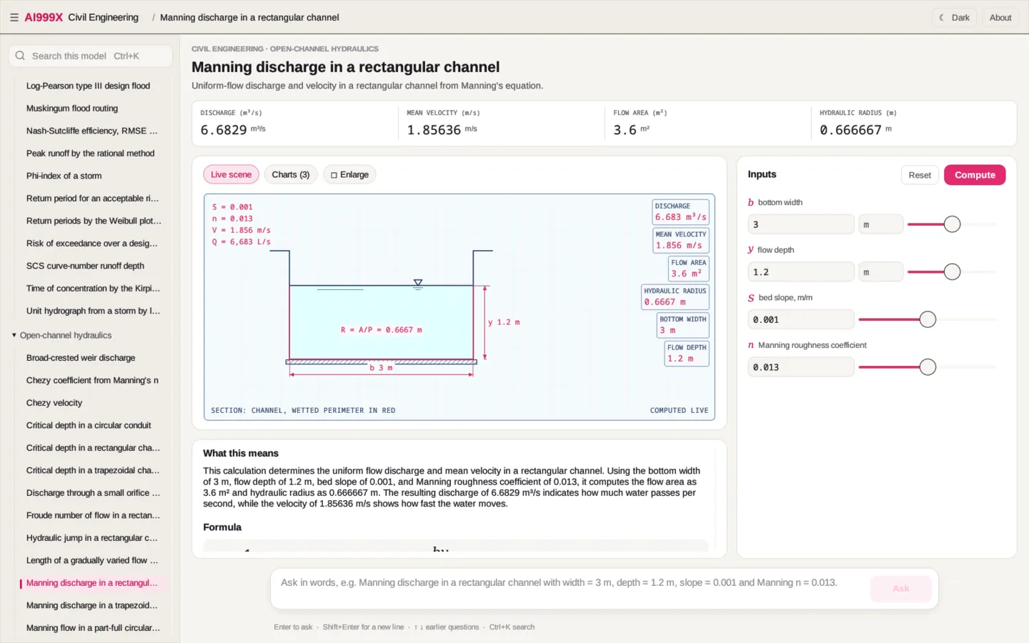
| Desktop app (Windows, Linux) | Windows · Linux |
Command line civil-engineering (Windows, Linux) |
Windows · Linux |
| Browser (any device) | Try it on the model page |
| Python 3.10+ | pip install civil-engineering-ai999x: on Windows and Linux (x86-64) pip installs the same compiled engine; on other systems (macOS, ARM) it installs a pure-Python build that gives the same answers |
From the Civil Engineering desktop app: every scene and chart is drawn from the computed answer.
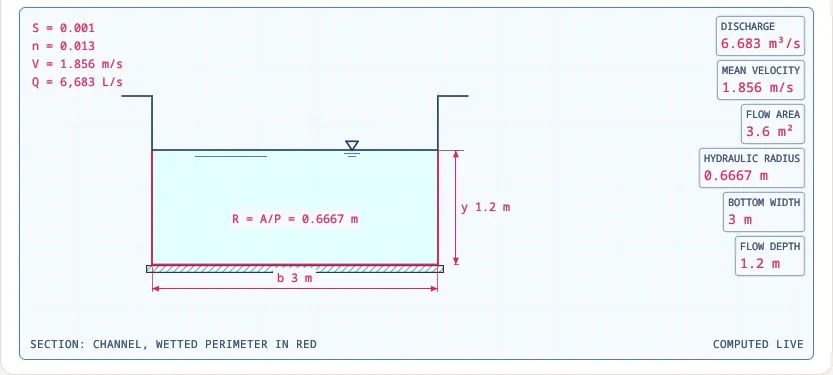 Manning discharge in a rectangular channel |
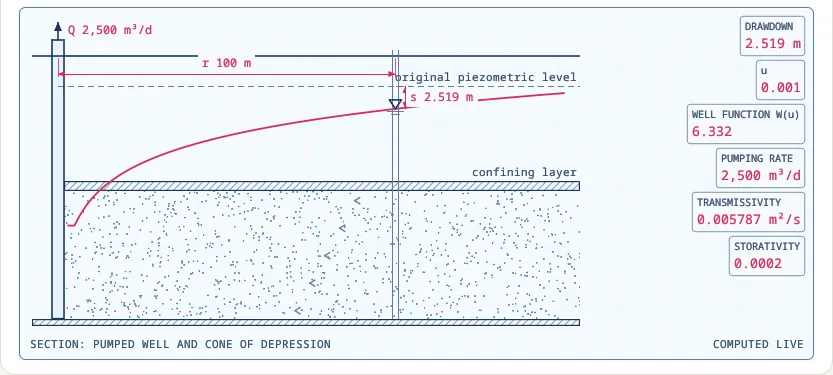 Theis drawdown around a pumped well |
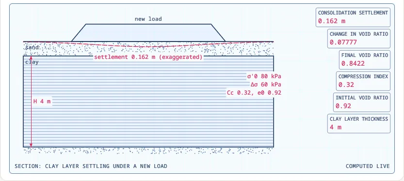 Primary consolidation settlement of a normally consolidated clay |
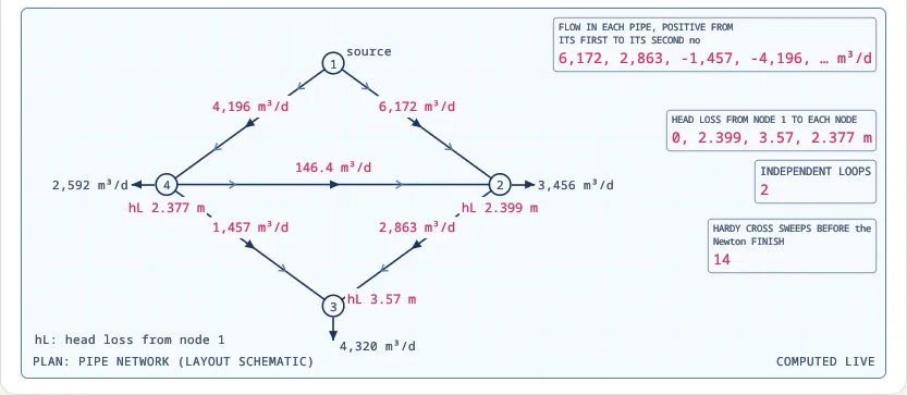 Pipe network flows by the Hardy Cross method (Hazen-Williams) |
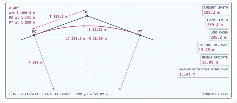 Elements of a simple horizontal circular curve |
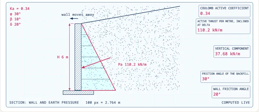 Coulomb active thrust on a rough wall with sloping backfill |
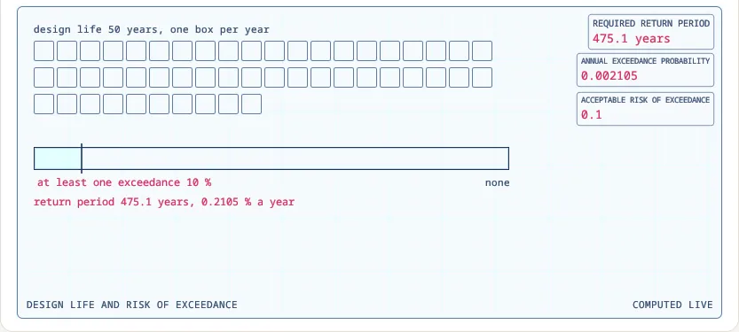 Return period for an acceptable risk over a design life |
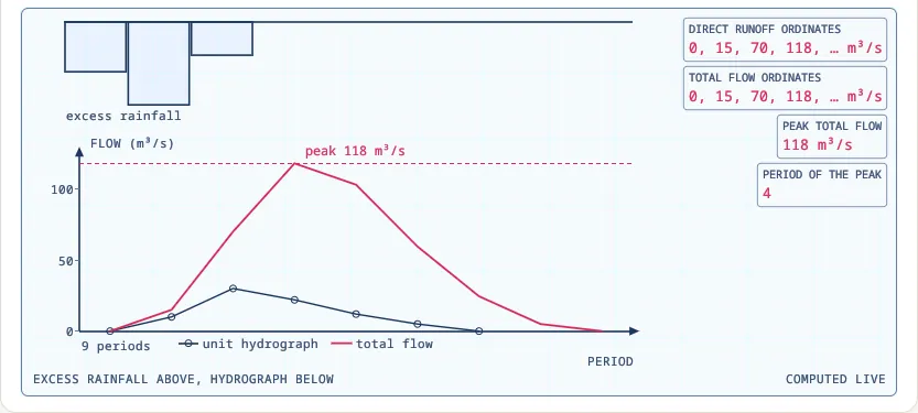 Direct runoff hydrograph by unit-hydrograph convolution |
Charts:
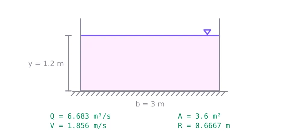 Manning discharge in a rectangular channel |
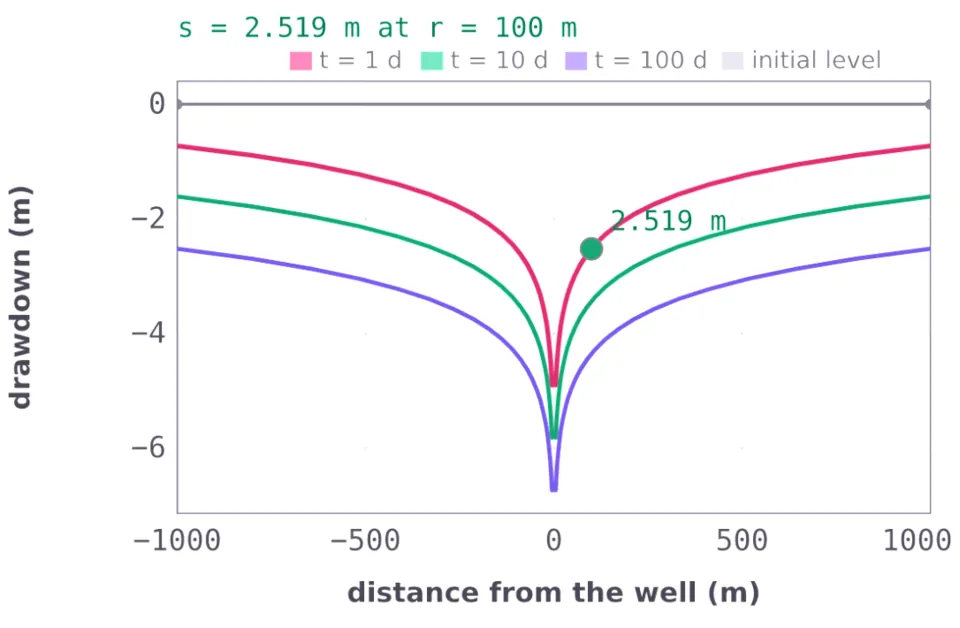 Theis drawdown around a pumped well |
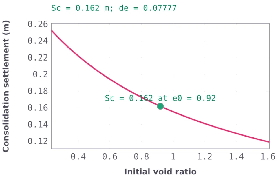 Primary consolidation settlement of a normally consolidated clay |
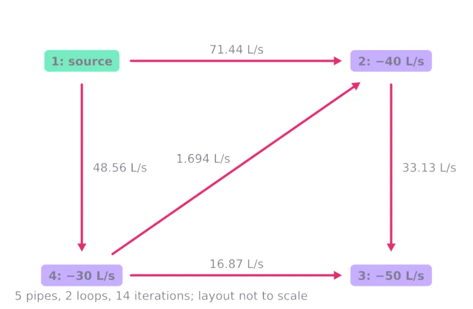 Pipe network flows by the Hardy Cross method (Hazen-Williams) |
Each question below was asked on this release; the comment under it is the line it printed.
import civil_engineering_ai999x as civil_engineering

a = civil_engineering.ask(
    "Broad crested weir discharge with discharge coefficient = 0.95, "
    "crest width = 5 m and head = 0.6 m."
)
print(a.outcome, a.values)
# SOLVED {'Q': 3.76372687638, 'yc': 0.4}

a = civil_engineering.ask(
    "Area from offsets with offsets = [0, 2.5, 3.5, 5, 4.6, 3.2, 0] "
    "and interval = 10 m."
)
print(a.outcome, a.values)
# SOLVED {'A_trapezoidal': 188.0, 'A_simpson': 196.666666667}

a = civil_engineering.ask(
    "Chezy coefficient from manning with Manning n = 0.013 and "
    "hydraulic radius = 0.75 m."
)
print(a.outcome, a.values)
# SOLVED {'C': 73.3218686921}

a = civil_engineering.ask(
    "Falling head permeability with standpipe diameter = 10 mm, sample "
    "diameter = 75 mm, sample length = 150 mm, initial head = 100 cm, "
    "final head = 60 cm and time = 600 s."
)
print(a.outcome, a.values)
# SOLVED {'K': 2.27033610563e-06, 'K_cm_s': 0.000227033610563}

a = civil_engineering.ask(
    "Chezy velocity with Chezy C = 55 m^0.5/s, hydraulic radius = 1.1 "
    "m and slope = 0.0004."
)
print(a.outcome, a.values)
# SOLVED {'V': 1.15368973299}

a = civil_engineering.ask(
    "Flow from head loss by hazen williams with head loss = 5 m, "
    "diameter = 300 mm, length = 1500 m and Hazen-Williams C = 110."
)
print(a.outcome, a.values)
# SOLVED {'Q': 0.0593636598191, 'V': 0.839823991132}

a = civil_engineering.ask(
    "Direct shear strength parameters with normal stresses = [50, 100, "
    "200] and shear stresses = [45, 73, 131]."
)
print(a.outcome, a.values)
# SOLVED {'phi': 29.8681357032, 'c': 16.0, 'tan_phi': 0.574285714286}

a = civil_engineering.ask(
    "Earthwork volume from cross sections with areas = [12.5, 18.2, "
    "25.6, 20.1, 15.8] and spacing = 20 m."
)
print(a.outcome, a.values)
# SOLVED {'V_end_area': 1561.0, 'V_prismoidal': 1551.33333333}

a = civil_engineering.ask(
    "Thiem unconfined conductivity with pumping rate = 1500 m^3/d, "
    "first distance = 20 m, second distance = 80 m, first head = 18.2 "
    "m and second head = 19.6 m."
)
print(a.outcome, a.values)
# SOLVED {'K': 0.0001447648968, 'K_m_d': 12.5076870835}

a = civil_engineering.ask(
    "Terzaghi bearing capacity with cohesion = 20 kPa, unit weight = "
    "18 kN/m^3, width = 2 m, depth = 1.5 m, Nc = 37.16, Nq = 22.46, "
    "Ngamma = 19.13 and footing shape = square."
)
print(a.outcome, a.values)
# SOLVED {'qu': 1848052.0, 'qa': 616017.333333, 'q_net': 1821052.0}

a = civil_engineering.ask(
    "Theis drawdown with pumping rate = 2500 m^3/d, transmissivity = "
    "500 m^2/d, storativity = 0.0002, distance = 100 m and time = 24 "
    "h."
)
print(a.outcome, a.values)
# SOLVED {'s': 2.51923946796, 'u': 0.001, 'W': 6.33153936414}

a = civil_engineering.ask(
    "Thick clay layer settlement with thickness = 10 m, top effective "
    "stress = 40 kPa, submerged unit weight = 8 kN/m^3, stress "
    "increase = 100 kPa, compression index = 0.45 and initial void "
    "ratio = 1.2."
)
print(a.outcome, a.values)
# SOLVED {'S': 0.753129074489, 'S_one_layer': 0.720373332501}

a = civil_engineering.ask(
    "Stress below a rectangular load with pressure = 200 kPa, width = "
    "2 m, length = 3 m and depth = 4 m."
)
print(a.outcome, a.values)
# SOLVED {'dsigma': 21414.5857952, 'I': 0.107072928976}

a = civil_engineering.ask(
    "Thiem confined transmissivity with pumping rate = 2500 m^3/d, "
    "first distance = 15 m, second distance = 60 m, first drawdown = "
    "2.8 m and second drawdown = 1.1 m."
)
print(a.outcome, a.values)
# SOLVED {'T': 0.00375537173462, 'T_m2_d': 324.464117872}

a = civil_engineering.ask(
    "Excess pore pressure during consolidation with initial excess "
    "pore pressure = 100 kPa, coefficient of consolidation = 2 m^2/yr, "
    "time = 1 yr, drainage path = 3 m and depth = 1.5 m."
)
print(a.outcome, a.values)
# SOLVED {'u': 52247.3336591, 'Uz': 0.477526663409, 'Tv': 0.222222222222}
Each command below was run with civil-engineering of this release; the lines under it are the answer it printed (the full answer goes on with the method, every input in SI units and the conditions it assumes).
$ civil-engineering solve coulomb_active_thrust phi=30 delta=20 beta=10 "gam=18000 N/m^3" "H=6 m"
Ka = 0.3400223954
Pa = 110167.2561 N/m
Pa_h = 103523.3576 N/m
Pa_v = 37679.42072 N/m

$ civil-engineering solve darcy_flow_layered_soil "H=[2]" "K=[1e-05]" "A=10 m^2" "dh=0.5 m"
Q = 2.5e-05 m^3/s
q = 2.5e-06 m/s
Kv = 1e-05 m/s
Kh = 1e-05 m/s
heads = [0.0] m

$ civil-engineering solve thiessen_polygon_rainfall "gx=[2, 8, 5]" "gy=[2, 3, 9]" "rain=[45, 60, 38]" "bx=[0, 10, 10, 0]" "by=[0, 0, 10, 10]"
mean = 47.23995192
areas = [29.6650641026,32.5608974359,37.7740384615]
weights = [0.296650641026,0.325608974359,0.377740384615]
arithmetic_mean = 47.66666667
catchment_area = 100

$ civil-engineering solve broad_crested_weir_discharge Cd=0.95 "b=5 m" "H=0.6 m"
Q = 3.763726876 m^3/s
yc = 0.4 m

$ civil-engineering solve parallel_pipes_hazen_williams "Q=0.3 m^3/s" "L=[800, 1200]" "D=[300, 400]" "C=[120, 110]"
hf = 7.944067369 m
flows = [0.116758581689,0.183241418311] m^3/s

$ civil-engineering solve degree_of_consolidation "cv=7.922021954e-08 m^2/s" "t=31557600 s" "Hdr=3 m"
Tv = 0.2777777778
U = 0.5913702173
U_percent = 59.13702173

$ civil-engineering solve area_from_offsets "offsets=[0, 2.5, 3.5, 5, 4.6, 3.2, 0]" "d=10 m"
A_trapezoidal = 188 m^2
A_simpson = 196.6666667 m^2

$ civil-engineering solve coulomb_passive_thrust phi=30 delta=15 beta=0 "gam=18000 N/m^3" "H=2 m"
Kp = 4.976500223
Pp = 179154.008 N/m
Pp_h = 173049.4832 N/m
Pp_v = 46368.46928 N/m

$ civil-engineering solve well_field_drawdown "wx=[0, 200]" "wy=[0, 0]" "Qs=[2000, 1500]" "T=0.00462962963 m^2/s" S=0.0003 "t=432000 s" "x0=100 m" "y0=50 m"
s = 4.935878027 m
parts = [2.82050172954,2.11537629715] m

$ civil-engineering solve unit_hydrograph_convolution "excess=[1.5, 2.5, 1]" "uh=[0, 10, 30, 22, 12, 5, 0]"
DRO = [0.0,15.0,70.0,118.0,103.0,59.5,24.5,5.0,0.0] m^3/s
total = [0.0,15.0,70.0,118.0,103.0,59.5,24.5,5.0,0.0] m^3/s
peak = 118 m^3/s
peak_period = 4

$ civil-engineering solve chezy_from_manning n=0.013 "R=0.75 m"
C = 73.32186869 m^0.5/s

$ civil-engineering solve hazen_williams_head_loss "Q=0.05 m^3/s" "D=0.3 m" "L=1000 m" C=120
hf = 2.064555214 m
V = 0.7073553026 m/s
Sf = 0.002064555214

$ civil-engineering solve coefficient_of_consolidation "Hdr=0.01 m" "t=750 s" U=0.5
cv = 2.623076527e-08 m^2/s
Tv = 0.1967307395
cv_m2_yr = 0.8277799981

$ civil-engineering solve traverse_bowditch_adjustment "az=[45, 135.01, 225, 315]" "d=[100, 100.02, 99.98, 100]"
misclosure_E = 0.01593938435 m
misclosure_N = -0.0123427325 m
linear_misclosure = 0.02015953915 m
precision = 19841.72341
E = [0.0,70.7066932726,141.415182997,70.7146629647] m
N = [0.0,70.7137638018,-0.020312884737,-70.7137638018] m

$ civil-engineering solve rankine_active_thrust phi=30 "gam=18000 N/m^3" "H=6 m"
Ka = 0.3333333333
sigma_base = 36000 Pa
Pa = 108000 N/m
z_crack = 0 m
ybar = 2 m
Every calculation, with its formula, a worked example and its figures: Civil Engineering on ai999x.com. Install guides for the app and the command line: https://www.ai999x.com/desktop-cli/.
Version 1.6.7 · License: Apache-2.0 · Author: Ibnul Jaif Farabi · Organization: AI999X · Contact: [email protected] · Support the project
The Future Is Self-Improving.